1 Chapter 1: Deryugina (2017) — Hurricane Hits and Government Transfers
Research Question: How do hurricanes affect non-disaster government transfer programs in the United States?
Data: County-year panel. Treatment hurricane is binary and non-absorbing (counties are treated for at most one year — a “one-shot” design). Outcome: log_curr_trans_ind_gov_pc (log non-disaster government transfers per capita).
1.1 T1: Verify One-Shot Design
* ssc install did_multiplegt_dyn, replace
copy "https://raw.githubusercontent.com/Credible-Answers/did_multiplegt_dyn_tutorial/main/data/deryugina_2017.dta" "deryugina_2017.dta", replace
use "deryugina_2017.dta", clear
egen total_hurricane = total(hurricane), by(county_fips)
sum total_hurricane
Variable | Obs Mean Std. dev. Min Max
-------------+---------------------------------------------------------
total_hurr~e | 49,698 .3163709 .4650642 0 1All counties have total_hurricane ∈ {0, 1} — confirming the one-shot design.
# install.packages(c("DIDmultiplegtDYN", "polars", "haven", "dplyr"))
library(haven)
library(dplyr)
library(DIDmultiplegtDYN)
library(polars)

load(url("https://raw.githubusercontent.com/Credible-Answers/did_multiplegt_dyn_tutorial/main/data/deryugina_2017.RData"))

df %>%
  group_by(county_fips) %>%
  summarise(total_hurricane = sum(hurricane, na.rm = TRUE)) %>%
  summarise(mean = mean(total_hurricane), sd = sd(total_hurricane),
            min = min(total_hurricane), max = max(total_hurricane))
# A tibble: 1 × 4
mean sd min max
<dbl> <dbl> <dbl> <dbl>
1 0.316 0.465 0 1All counties have total_hurricane ∈ {0, 1} — confirming the one-shot design.
# pip install py-did-multiplegt-dyn pandas pyarrow
import pandas as pd
import polars as pl
from did_multiplegt_dyn import DidMultiplegtDyn

df = pd.read_parquet("https://raw.githubusercontent.com/Credible-Answers/did_multiplegt_dyn_tutorial/main/data/deryugina_2017.parquet")

total = df.groupby("county_fips")["hurricane"].sum().reset_index(name="total_hurricane")
print(total["total_hurricane"].describe())
count 4518.000000
mean 0.316371
std 0.465064
min 0.000000
max 1.000000All counties have total_hurricane ∈ {0, 1} — confirming the one-shot design.
1.2 T2: Non-Normalized Event-Study Effects (No Controls)
* ssc install did_multiplegt_dyn, replace
copy "https://raw.githubusercontent.com/Credible-Answers/did_multiplegt_dyn_tutorial/main/data/deryugina_2017.dta" "deryugina_2017.dta", replace
use "deryugina_2017.dta", clear

did_multiplegt_dyn log_curr_trans_ind_gov_pc county_fips year hurricane, effects(11) placebo(11) cluster(county_fips)
--------------------------------------------------------------------------------
Estimation of treatment effects: Event-study effects
--------------------------------------------------------------------------------
| Estimate SE LB CI UB CI N Switchers
-------------+------------------------------------------------------------------
Effect_1 | .0108629 .001617 .0076937 .0140321 14240 361
Effect_2 | .0127918 .0023651 .0081563 .0174273 13953 361
Effect_3 | .0158005 .0030075 .0099059 .021695 13766 361
Effect_4 | .0163886 .003393 .0097385 .0230388 13620 361
Effect_5 | .0230699 .0038968 .0154322 .0307076 13462 361
Effect_6 | .0268285 .0042508 .0184972 .0351598 13253 361
Effect_7 | .0377147 .0044926 .0289095 .04652 13038 361
Effect_8 | .0392922 .0050394 .0294151 .0491694 12929 361
Effect_9 | .035109 .0055185 .0242929 .0459251 12840 361
Effect_10 | .0494016 .006029 .0375849 .0612182 12741 361
Effect_11 | .0518123 .0061055 .0398457 .0637788 12619 361
--------------------------------------------------------------------------------
Test of joint nullity of the effects : p-value = 0
Av_tot_eff | .3190721 .0406001 .2394973 .3986468 31470 3971
Average number of time periods over which a treatment's effect is accumulated = 11
Placebo_1 | -.0055903 .0013173 -.008172 -.0030085 14154 361
Placebo_2 | -.0083554 .0020689 -.0124104 -.0043003 13826 361
Placebo_3 | -.0128183 .002977 -.0186532 -.0069834 13567 361
Placebo_4 | -.009143 .0033686 -.0157454 -.0025406 13302 361
Placebo_5 | -.0075546 .0039816 -.0153585 .0002493 13005 361
Placebo_6 | -.0073115 .0043748 -.015886 .001263 12682 361
Placebo_7 | -.0079583 .0047566 -.0172812 .0013645 12431 361
Placebo_8 | -.008841 .0053184 -.0192648 .0015829 12214 361
Placebo_9 | -.0143816 .0058363 -.0258204 -.0029427 11829 361
Placebo_10 | -.0086498 .0061281 -.0206606 .0033611 10807 299
Placebo_11 | -.0035924 .0066904 -.0167053 .0095206 10012 282
--------------------------------------------------------------------------------
Test of joint nullity of the placebos : p-value = 1.517e-06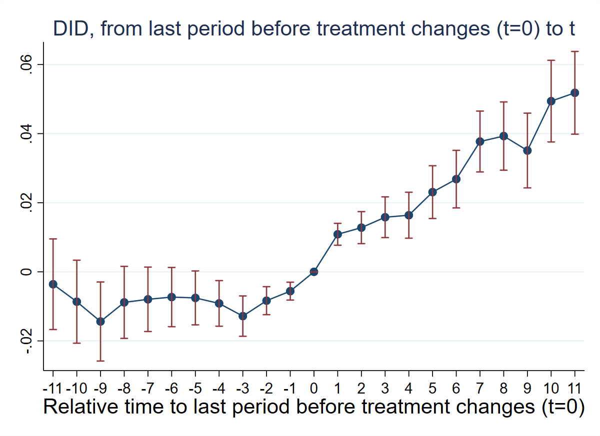
# install.packages(c("DIDmultiplegtDYN", "polars", "ggplot2"))
library(DIDmultiplegtDYN)
library(polars)
library(ggplot2)

load(url("https://raw.githubusercontent.com/Credible-Answers/did_multiplegt_dyn_tutorial/main/data/deryugina_2017.RData"))

res_t2 <- did_multiplegt_dyn(
  df        = df,
  outcome   = "log_curr_trans_ind_gov_pc",
  group     = "county_fips",
  time      = "year",
  treatment = "hurricane",
  effects   = 11,
  placebo   = 11,
  cluster   = "county_fips"
)
print(res_t2)
res_t2$plot
----------------------------------------------------------------------
Estimation of treatment effects: Event-study effects
----------------------------------------------------------------------
Estimate SE LB CI UB CI N Switchers
Effect_1 0.01086 0.00162 0.00769 0.01403 14,240 361
Effect_2 0.01279 0.00237 0.00816 0.01743 13,953 361
Effect_3 0.01580 0.00301 0.00991 0.02170 13,766 361
Effect_4 0.01639 0.00339 0.00974 0.02304 13,620 361
Effect_5 0.02307 0.00390 0.01543 0.03071 13,462 361
Effect_6 0.02683 0.00425 0.01850 0.03516 13,253 361
Effect_7 0.03771 0.00449 0.02891 0.04652 13,038 361
Effect_8 0.03929 0.00504 0.02942 0.04917 12,929 361
Effect_9 0.03511 0.00552 0.02429 0.04593 12,840 361
Effect_10 0.04940 0.00603 0.03758 0.06122 12,741 361
Effect_11 0.05181 0.00611 0.03985 0.06378 12,619 361
Test of joint nullity of the effects : p-value = 0.0000000
Av_tot_eff | 0.31907 0.04060 0.23950 0.39865 31,470 3,971
Average number of time periods over which a treatment effect is accumulated: 11
Placebo_1 -0.00559 0.00132 -0.00817 -0.00301 14,154 361
Placebo_2 -0.00836 0.00207 -0.01241 -0.00430 13,826 361
Placebo_3 -0.01282 0.00298 -0.01865 -0.00698 13,567 361
Placebo_4 -0.00914 0.00337 -0.01575 -0.00254 13,302 361
Placebo_5 -0.00755 0.00398 -0.01536 0.00025 13,005 361
Placebo_6 -0.00731 0.00437 -0.01589 0.00126 12,682 361
Placebo_7 -0.00796 0.00476 -0.01728 0.00136 12,431 361
Placebo_8 -0.00884 0.00532 -0.01926 0.00158 12,214 361
Placebo_9 -0.01438 0.00584 -0.02582 -0.00294 11,829 361
Placebo_10 -0.00865 0.00613 -0.02066 0.00336 10,807 299
Placebo_11 -0.00359 0.00669 -0.01671 0.00952 10,012 282
Test of joint nullity of the placebos : p-value = 0.0000015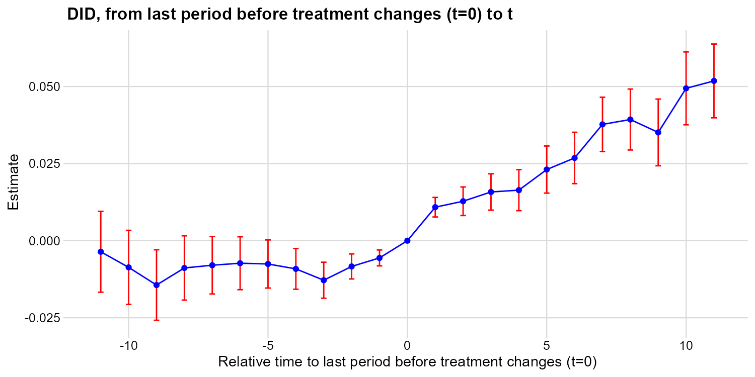
# pip install py-did-multiplegt-dyn pandas pyarrow
import pandas as pd
import polars as pl
import matplotlib
matplotlib.use('Agg')
import matplotlib.pyplot as plt
from did_multiplegt_dyn import DidMultiplegtDyn

df = pd.read_parquet("https://raw.githubusercontent.com/Credible-Answers/did_multiplegt_dyn_tutorial/main/data/deryugina_2017.parquet")

res_t2 = DidMultiplegtDyn(
    df=pl.from_pandas(df),
    outcome="log_curr_trans_ind_gov_pc", group="county_fips",
    time="year", treatment="hurricane",
    effects=11, placebo=11, cluster="county_fips"
)
res_t2.fit()
res_t2.summary()
res_t2.plot()
plt.savefig("ch09_fig1_hurricane_nocontrols_py.png", dpi=150, bbox_inches="tight")
plt.close()
================================================================================
Estimation of treatment effects: Event-study effects
================================================================================
Block Estimate SE LB CI UB CI N Switchers
Effect_1 0.010863 0.001617 0.007694 0.014032 14240.0 361.0
Effect_2 0.012792 0.002365 0.008156 0.017427 13953.0 361.0
Effect_3 0.015800 0.003007 0.009906 0.021695 13766.0 361.0
Effect_4 0.016389 0.003393 0.009739 0.023039 13620.0 361.0
Effect_5 0.023070 0.003897 0.015432 0.030708 13462.0 361.0
Effect_6 0.026829 0.004251 0.018497 0.035160 13253.0 361.0
Effect_7 0.037715 0.004493 0.028909 0.046520 13038.0 361.0
Effect_8 0.039292 0.005039 0.029415 0.049169 12929.0 361.0
Effect_9 0.035109 0.005519 0.024293 0.045925 12840.0 361.0
Effect_10 0.049402 0.006029 0.037585 0.061218 12741.0 361.0
Effect_11 0.051812 0.006105 0.039846 0.063779 12619.0 361.0
Average_Total_Effect 0.319072 0.040600 0.239497 0.398647 31470.0 3971.0
Placebo_1 -0.005590 0.001317 -0.008172 -0.003008 14154.0 361.0
Placebo_2 -0.008355 0.002069 -0.012410 -0.004300 13826.0 361.0
Placebo_3 -0.012818 0.002977 -0.018653 -0.006983 13567.0 361.0
Placebo_4 -0.009143 0.003369 -0.015745 -0.002541 13302.0 361.0
Placebo_5 -0.007555 0.003982 -0.015359 0.000249 13005.0 361.0
Placebo_6 -0.007312 0.004375 -0.015886 0.001263 12682.0 361.0
Placebo_7 -0.007958 0.004757 -0.017281 0.001365 12431.0 361.0
Placebo_8 -0.008841 0.005318 -0.019265 0.001583 12214.0 361.0
Placebo_9 -0.014382 0.005836 -0.025820 -0.002943 11829.0 361.0
Placebo_10 -0.008650 0.006128 -0.020661 0.003361 10807.0 299.0
Placebo_11 -0.003592 0.006690 -0.016705 0.009521 10012.0 282.0
================================================================================
Test of joint nullity of the effects: p-value = 0.000000
Test of joint nullity of the placebos: p-value = 0.000002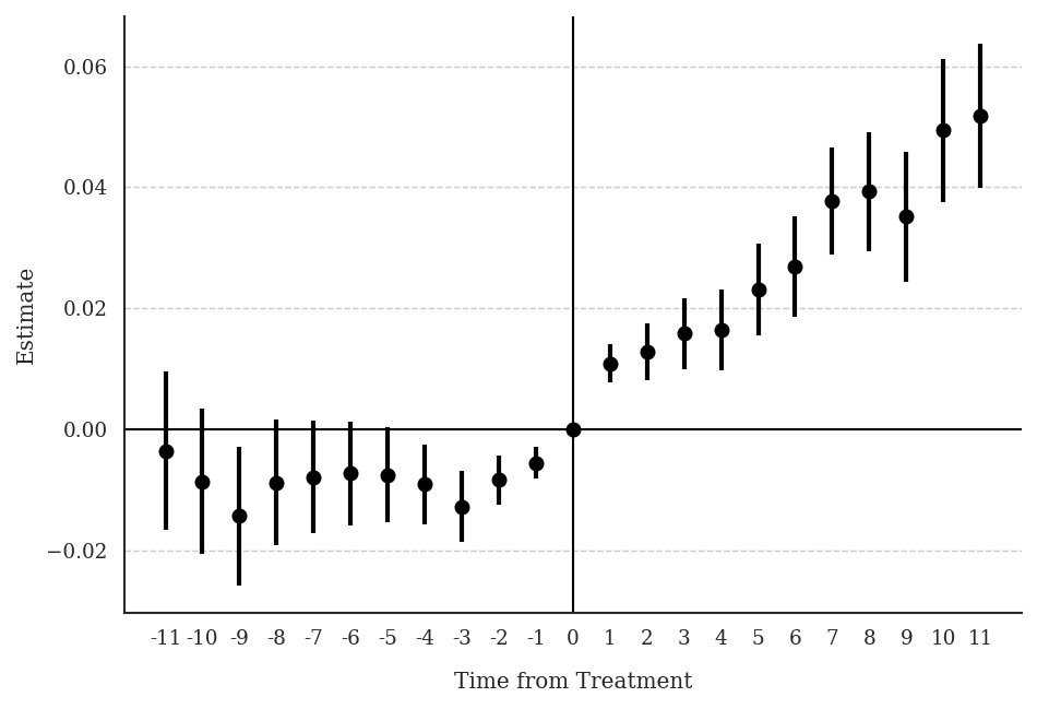
Interpretation: Effects are positive and increasing — hurricanes raise non-disaster transfers by ~1% in the short run and ~5% in the long run. The pre-trend test is highly significant (p ≈ 1.5e-06), suggesting a differential trend starting ~4 periods before treatment. The parallel-trends assumption is likely violated without controls.
1.3 T3: Non-Normalized Event-Study Effects (With County-Level Controls)
* ssc install did_multiplegt_dyn, replace
copy "https://raw.githubusercontent.com/Credible-Answers/did_multiplegt_dyn_tutorial/main/data/deryugina_2017.dta" "deryugina_2017.dta", replace
use "deryugina_2017.dta", clear

local vars coastal land_area1970 log_pop1969 frac_young1969 frac_old1969 frac_black1969 log_wage_pc1969 emp_rate1969
local controls
foreach v of local vars {
    gen `v'_year = `v' * year
    local controls `controls' `v'_year
}

did_multiplegt_dyn log_curr_trans_ind_gov_pc county_fips year hurricane, effects(11) placebo(11) cluster(county_fips) controls(`controls')
--------------------------------------------------------------------------------
Estimation of treatment effects: Event-study effects
--------------------------------------------------------------------------------
| Estimate SE LB CI UB CI N Switchers
-------------+------------------------------------------------------------------
Effect_1 | .0092419 .0015835 .0061383 .0123456 14077 361
Effect_2 | .0095925 .0022712 .0051409 .0140441 13794 361
Effect_3 | .0109771 .0028662 .0053594 .0165948 13609 361
Effect_4 | .0097365 .0032466 .0033733 .0160998 13464 361
Effect_5 | .0144296 .0037154 .0071476 .0217116 13305 361
Effect_6 | .0164425 .0040354 .0085333 .0243517 13097 361
Effect_7 | .0254598 .0042959 .0170399 .0338797 12884 361
Effect_8 | .0251647 .0048611 .0156371 .0346923 12775 361
Effect_9 | .0192179 .0053476 .0087368 .0296989 12685 361
Effect_10 | .031657 .0058645 .0201628 .0431512 12587 361
Effect_11 | .0317402 .0059652 .0200487 .0434317 12465 361
--------------------------------------------------------------------------------
Test of joint nullity of the effects : p-value = 0
Av_tot_eff | .2036597 .038535 .1281326 .2791869 31123 3971
Placebo_1 | -.0039173 .0013091 -.006483 -.0013515 14000 361
Placebo_2 | -.0051001 .0020352 -.009089 -.0011111 13679 361
Placebo_3 | -.0077511 .0029252 -.0134844 -.0020179 13430 361
Placebo_4 | -.0024941 .003301 -.0089639 .0039757 13181 361
Placebo_5 | .0011302 .00376 -.0062391 .0084996 12893 361
Placebo_6 | .003105 .0040325 -.0047987 .0110086 12577 361
Placebo_7 | .004438 .0043775 -.0041417 .0130177 12337 361
Placebo_8 | .0054782 .0048862 -.0040986 .0150551 12126 361
Placebo_9 | .0018036 .0052736 -.0085325 .0121397 11749 361
Placebo_10 | .0102888 .0056563 -.0007973 .0213749 10734 299
Placebo_11 | .0177286 .0060115 .0059462 .029511 9948 282
--------------------------------------------------------------------------------
Test of joint nullity of the placebos : p-value = 3.280e-07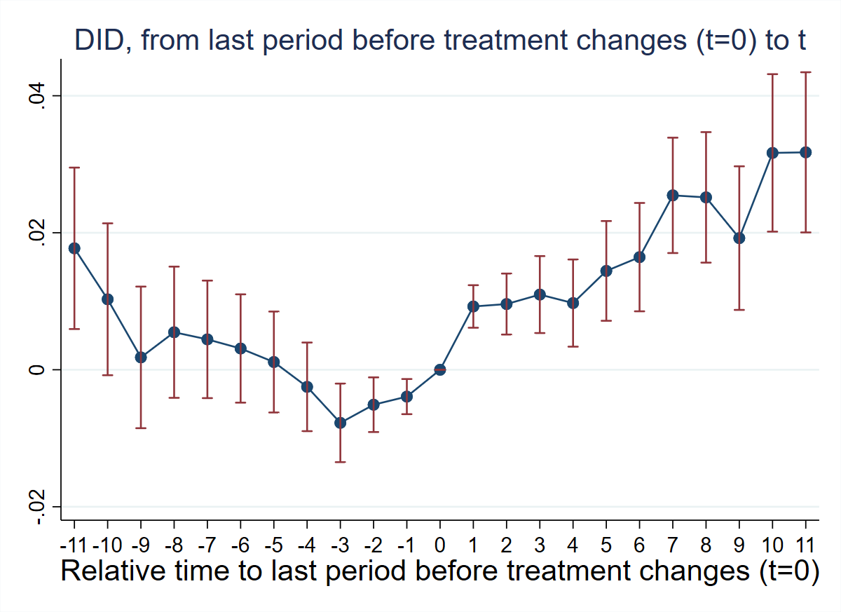
# install.packages(c("DIDmultiplegtDYN", "polars", "ggplot2"))
library(DIDmultiplegtDYN)
library(polars)
library(ggplot2)

load(url("https://raw.githubusercontent.com/Credible-Answers/did_multiplegt_dyn_tutorial/main/data/deryugina_2017.RData"))

vars <- c("coastal", "land_area1970", "log_pop1969", "frac_young1969",
          "frac_old1969", "frac_black1969", "log_wage_pc1969", "emp_rate1969")
for (v in vars) df[[paste0(v, "_year")]] <- df[[v]] * df$year
controls_list <- paste0(vars, "_year")

res_t3 <- did_multiplegt_dyn(
  df        = df,
  outcome   = "log_curr_trans_ind_gov_pc",
  group     = "county_fips",
  time      = "year",
  treatment = "hurricane",
  effects   = 11,
  placebo   = 11,
  cluster   = "county_fips",
  controls  = controls_list
)
print(res_t3)
res_t3$plot
----------------------------------------------------------------------
Estimation of treatment effects: Event-study effects
----------------------------------------------------------------------
Estimate SE LB CI UB CI N Switchers
Effect_1 0.00924 0.00158 0.00614 0.01235 14,077 361
Effect_2 0.00959 0.00227 0.00514 0.01404 13,794 361
Effect_3 0.01098 0.00287 0.00536 0.01659 13,609 361
Effect_4 0.00974 0.00325 0.00337 0.01610 13,464 361
Effect_5 0.01443 0.00372 0.00715 0.02171 13,305 361
Effect_6 0.01644 0.00404 0.00853 0.02435 13,097 361
Effect_7 0.02546 0.00430 0.01704 0.03388 12,884 361
Effect_8 0.02517 0.00486 0.01564 0.03469 12,775 361
Effect_9 0.01922 0.00535 0.00874 0.02970 12,685 361
Effect_10 0.03166 0.00586 0.02016 0.04315 12,587 361
Effect_11 0.03174 0.00597 0.02005 0.04343 12,465 361
Test of joint nullity of the effects : p-value = 0.0000
Av_tot_eff | 0.20366 0.03853 0.12814 0.27919 31,123 3,971
Average number of time periods over which a treatment effect is accumulated: 11.0000
Placebo_1 -0.00392 0.00131 -0.00648 -0.00135 14,000 361
Placebo_2 -0.00510 0.00204 -0.00909 -0.00111 13,679 361
Placebo_3 -0.00775 0.00293 -0.01348 -0.00202 13,430 361
Placebo_4 -0.00249 0.00330 -0.00896 0.00398 13,181 361
Placebo_5 0.00113 0.00376 -0.00624 0.00850 12,893 361
Placebo_6 0.00310 0.00403 -0.00480 0.01101 12,577 361
Placebo_7 0.00444 0.00438 -0.00414 0.01302 12,337 361
Placebo_8 0.00548 0.00489 -0.00410 0.01505 12,126 361
Placebo_9 0.00180 0.00527 -0.00853 0.01214 11,749 361
Placebo_10 0.01029 0.00566 -0.00080 0.02137 10,734 299
Placebo_11 0.01773 0.00601 0.00595 0.02951 9,948 282
Test of joint nullity of the placebos : p-value = 0.0000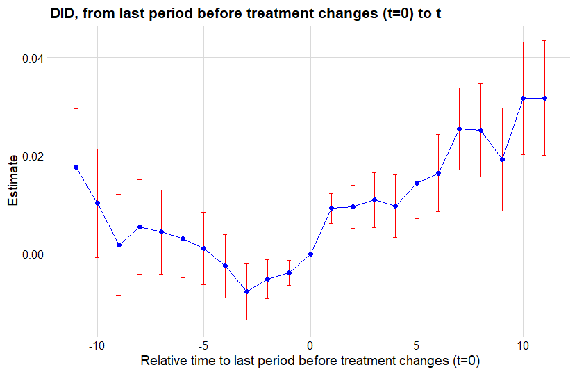
# pip install py-did-multiplegt-dyn pandas pyarrow
import pandas as pd
import polars as pl
import matplotlib
matplotlib.use('Agg')
import matplotlib.pyplot as plt
from did_multiplegt_dyn import DidMultiplegtDyn

df = pd.read_parquet("https://raw.githubusercontent.com/Credible-Answers/did_multiplegt_dyn_tutorial/main/data/deryugina_2017.parquet")

vars_list = ["coastal", "land_area1970", "log_pop1969", "frac_young1969",
             "frac_old1969", "frac_black1969", "log_wage_pc1969", "emp_rate1969"]
for v in vars_list:
    df[f"{v}_year"] = df[v] * df["year"]
controls_list = [f"{v}_year" for v in vars_list]

res_t3 = DidMultiplegtDyn(
    df=pl.from_pandas(df),
    outcome="log_curr_trans_ind_gov_pc", group="county_fips",
    time="year", treatment="hurricane",
    effects=11, placebo=11, cluster="county_fips",
    controls=controls_list
)
res_t3.fit()
res_t3.summary()
res_t3.plot()
plt.savefig("ch09_fig2_hurricane_controls_py.png", dpi=150, bbox_inches="tight")
plt.close()
================================================================================
Estimation of treatment effects: Event-study effects
================================================================================
Block Estimate SE LB CI UB CI N Switchers
Effect_1 0.009242 0.001584 0.006138 0.012346 14077.0 361.0
Effect_2 0.009593 0.002271 0.005141 0.014044 13794.0 361.0
Effect_3 0.010977 0.002866 0.005360 0.016595 13609.0 361.0
Effect_4 0.009737 0.003247 0.003374 0.016100 13464.0 361.0
Effect_5 0.014430 0.003715 0.007148 0.021712 13305.0 361.0
Effect_6 0.016443 0.004035 0.008534 0.024352 13097.0 361.0
Effect_7 0.025460 0.004296 0.017040 0.033880 12884.0 361.0
Effect_8 0.025165 0.004861 0.015638 0.034693 12775.0 361.0
Effect_9 0.019219 0.005348 0.008738 0.029699 12685.0 361.0
Effect_10 0.031658 0.005864 0.020163 0.043152 12587.0 361.0
Effect_11 0.031741 0.005965 0.020050 0.043433 12465.0 361.0
Average_Total_Effect 0.203664 0.038535 0.128137 0.279191 31123.0 3971.0
Placebo_1 -0.003917 0.001309 -0.006483 -0.001352 14000.0 361.0
Placebo_2 -0.005100 0.002035 -0.009089 -0.001111 13679.0 361.0
Placebo_3 -0.007752 0.002925 -0.013485 -0.002018 13430.0 361.0
Placebo_4 -0.002494 0.003301 -0.008964 0.003975 13181.0 361.0
Placebo_5 0.001130 0.003760 -0.006240 0.008499 12893.0 361.0
Placebo_6 0.003104 0.004033 -0.004799 0.011008 12577.0 361.0
Placebo_7 0.004437 0.004377 -0.004142 0.013017 12337.0 361.0
Placebo_8 0.005478 0.004886 -0.004099 0.015054 12126.0 361.0
Placebo_9 0.001803 0.005274 -0.008533 0.012139 11749.0 361.0
Placebo_10 0.010288 0.005656 -0.000798 0.021374 10734.0 299.0
Placebo_11 0.017728 0.006011 0.005946 0.029510 9948.0 282.0
================================================================================
Test of joint nullity of the effects: p-value = 0.000000
Test of joint nullity of the placebos: p-value = 0.000000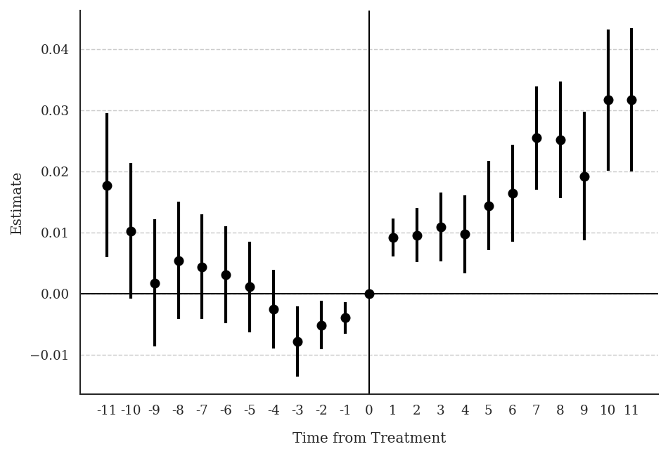
Interpretation: After including controls, effects remain positive and significant (Av_tot_eff ≈ 0.204 vs. 0.319 without controls). Pre-trends improve but the joint test remains significant (p ≈ 3.3e-07), suggesting a persistent differential trend even after conditioning on covariates.