Chapter 3: The Classical DID Design
Overview
Dataset: Moser & Voena (2012) — moser_voena_didtextbook.dta(Stata), moser_voena_didtextbook.RData (R), moser_voena_didtextbook.parquet (Python)
The Trading with the Enemy Act (TWEA) allowed US firms to use German-owned patents. Treatment (\(D_{g,t}\)) equals 1 for the 336 subclasses that received German patents, starting in 1919. The dataset contains 289,920 observations (7,248 subclasses × 40 years).
Panel View
* ssc install panelview, replace
copy "https://raw.githubusercontent.com/Credible-Answers/did_book/main/cc_xd_didtextbook_2025_9_30/Data%20sets/Moser%20and%20Voena%202012/moser_voena_didtextbook.dta" "moser_voena_didtextbook.dta", replace
use "moser_voena_didtextbook.dta", clear
panelview patents twea, i(subclass) t(year) type(treat) title("Treatment Status: Moser & Voena (2012)") ylabel(none) ytitle("")
graph export "figures/ch03_panelview_stata.png", replace width(1200)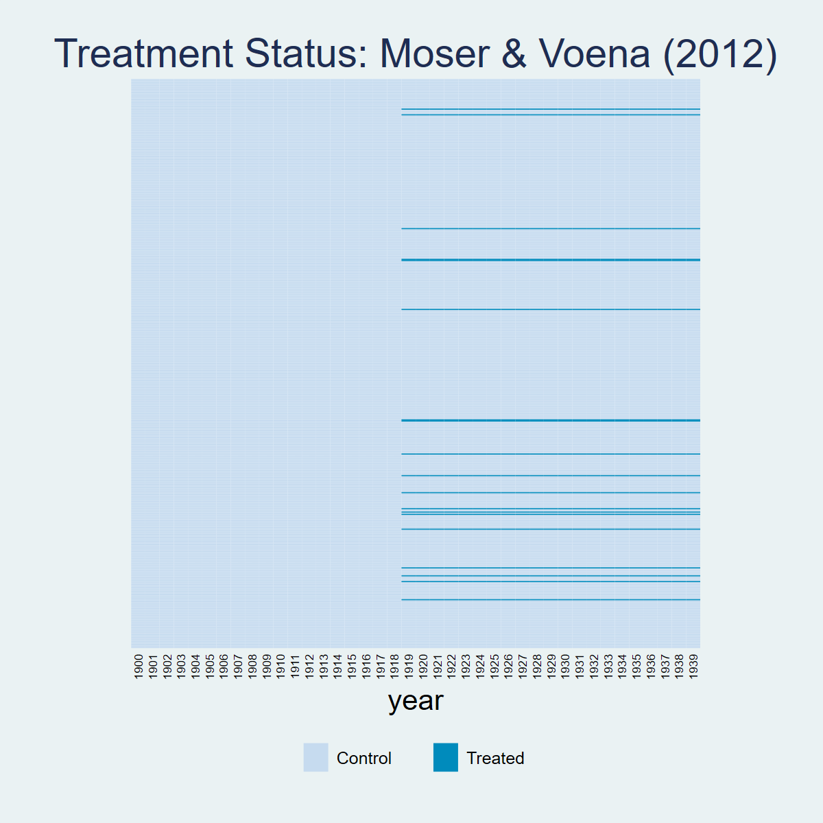
library(panelView)
load(url("https://raw.githubusercontent.com/Credible-Answers/did_book/main/cc_xd_didtextbook_2025_9_30/Data%20sets/Moser%20and%20Voena%202012/moser_voena_didtextbook.RData"))
png("figures/ch03_panelview_R.png", width = 1000, height = 600)
panelview(patents ~ twea, data = df, index = c("subclass", "year"), type = "treat",
          main = "Moser & Voena (2012)", ylab = "")
dev.off()
import pandas as pd
import matplotlib.pyplot as plt
import matplotlib.colors as mcolors
from matplotlib.patches import Patch

df = pd.read_parquet("https://raw.githubusercontent.com/Credible-Answers/did_book/main/cc_xd_didtextbook_2025_9_30/Data%20sets/Moser%20and%20Voena%202012/moser_voena_didtextbook.parquet")
pv = df.pivot_table(index="subclass", columns="year", values="twea", aggfunc="first")
pv_sorted = pv.loc[pv.mean(axis=1).sort_values(ascending=False).index]
cmap = mcolors.ListedColormap(["#D4E6F1", "#00AAAA"])
fig, ax = plt.subplots(figsize=(12, 10))
ax.imshow(pv_sorted.values, aspect="auto", cmap=cmap, interpolation="nearest", vmin=0, vmax=1)
for i in range(0, len(pv_sorted), 10):
    ax.axhline(y=i - 0.5, color="white", linewidth=0.15)
ax.set_xticks(range(0, len(pv_sorted.columns), 1))
ax.set_xticklabels([int(c) for c in pv_sorted.columns], rotation=45, ha="right", fontsize=8)
ax.set_yticks([])
ax.set_xlabel("year")
ax.set_title("Treatment Status: Moser & Voena (2012)", fontsize=16)
ax.legend(handles=[Patch(facecolor="#D4E6F1", edgecolor="gray", label="Control"),
                   Patch(facecolor="#00AAAA", edgecolor="gray", label="Treated")],
          loc="lower center", bbox_to_anchor=(0.5, -0.12), ncol=2)
plt.tight_layout()
plt.savefig("figures/ch03_panelview_Python.png", dpi=150, bbox_inches="tight")
plt.show()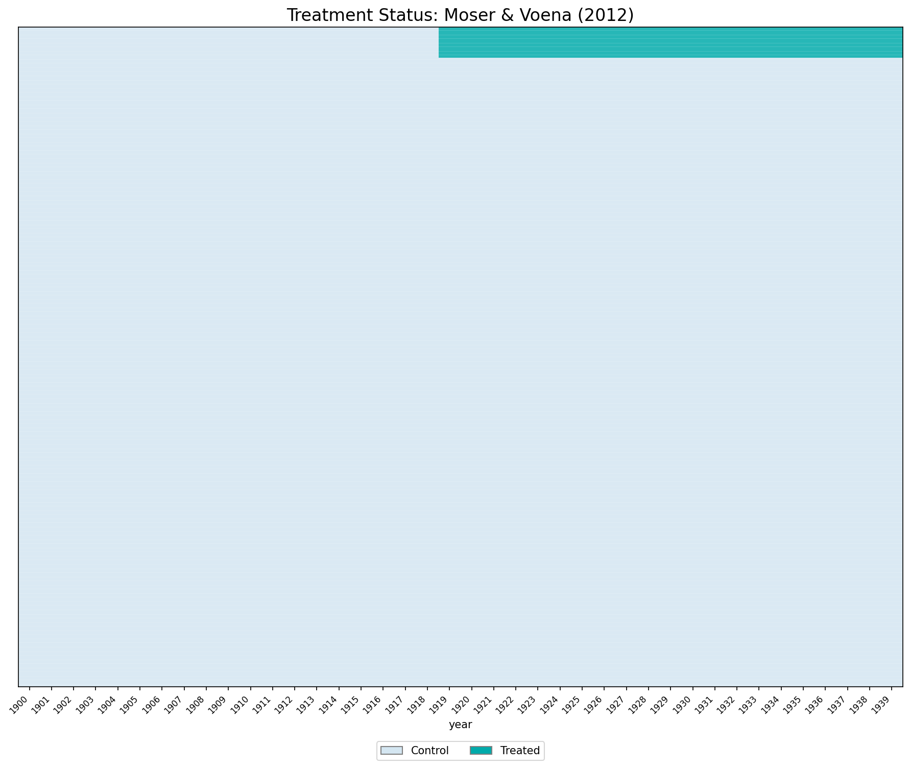
CQ#1: Static TWFE Regression
Using the
moser_voena_didtextbookdataset, run the TWFE regression of the number of patents in subclass \(g\) and year \(t\) on subclass and year FEs and thetweatreatment, clustering standard errors at the subclass level.
* ssc install reghdfe, replace
copy "https://raw.githubusercontent.com/Credible-Answers/did_book/main/cc_xd_didtextbook_2025_9_30/Data%20sets/Moser%20and%20Voena%202012/moser_voena_didtextbook.dta" "moser_voena_didtextbook.dta", replace
use "moser_voena_didtextbook.dta", clear

* Option 1: xtreg
xtreg patents twea i.year, fe i(subclass) robust cluster(subclass)

* Option 2: reghdfe
reghdfe patents twea, absorb(subclass year) cluster(subclass)
Both commands yield the same coefficient:
(Std. err. adjusted for 7,248 clusters in subclass)
------------------------------------------------------------------------------
| Robust
patents | Coefficient std. err. t P>|t| [95% conf. interval]
-------------+----------------------------------------------------------------
twea | .2882615 .0388871 7.41 0.000 .2120315 .3644915
------------------------------------------------------------------------------library(fixest); library(haven)
options(digits=7)
load(url("https://raw.githubusercontent.com/Credible-Answers/did_book/main/cc_xd_didtextbook_2025_9_30/Data%20sets/Moser%20and%20Voena%202012/moser_voena_didtextbook.RData"))
# Example 1
summary(feols(patents ~ twea + i(year) | subclass, data = df, cluster = ~subclass))
# Example 2
summary(feols(patents ~ twea | subclass + year, data = df, cluster = ~subclass))Example 1 (feols with i(year)):
Estimate Std. Error t value Pr(>|t|)
twea 0.288262 0.038887 7.412783 1.3770e-13 ***
Example 2 (feols with subclass + year):
Estimate Std. Error t value Pr(>|t|)
twea 0.288262 0.038887 7.41278 1.377e-13 ***import pandas as pd
import pyfixest as pf
df = pd.read_parquet("https://raw.githubusercontent.com/Credible-Answers/did_book/main/cc_xd_didtextbook_2025_9_30/Data%20sets/Moser%20and%20Voena%202012/moser_voena_didtextbook.parquet")
# Example 1
m1 = pf.feols('patents ~ twea + i(year) | subclass', data=df, vcov={'CRV1': 'subclass'})
c1 = m1.coef(); s1 = m1.se(); t1 = m1.tstat(); p1 = m1.pvalue()
for name in c1.index:
print(f"{name:>20s} | {c1[name]:>12.7f} {s1[name]:>10.7f} {t1[name]:>8.2f} {p1[name]:>8.4f}")
# Example 2
m2 = pf.feols('patents ~ twea | subclass + year', data=df, vcov={'CRV1': 'subclass'})
c2 = m2.coef(); s2 = m2.se(); t2 = m2.tstat(); p2 = m2.pvalue()
print("\n--- Example 2 ---")
for name in c2.index:
print(f"{name:>20s} | {c2[name]:>12.7f} {s2[name]:>10.7f} {t2[name]:>8.2f} {p2[name]:>8.4f}")Example 1:
twea | 0.2882615 0.0388871 7.41 0.0000
C(year)[T.1901] | 0.0059327 0.0077529 0.77 0.4442
...
Example 2:
twea | 0.2882615 0.0388871 7.41 0.0000Result: The coefficient on twea is 0.28826 (\(t = 7.41\), \(p < 0.001\)) across all three languages. Compulsory licensing has a positive and significant effect on US innovation.
CQ#2: Equivalence between Static TWFE and DID
Verify that \(\hat{\beta}_{fe}\) equals the coefficient on
tweain a regression on the treatment group indicator, the post indicator, andtwea.
copy "https://raw.githubusercontent.com/Credible-Answers/did_book/main/cc_xd_didtextbook_2025_9_30/Data%20sets/Moser%20and%20Voena%202012/moser_voena_didtextbook.dta" "moser_voena_didtextbook.dta", replace
use "moser_voena_didtextbook.dta", clear
reg patents treatmentgroup post twea, cluster(subclass)
(Std. err. adjusted for 7,248 clusters in subclass)
--------------------------------------------------------------------------------
| Robust
patents | Coefficient std. err. t P>|t| [95% conf. interval]
---------------+----------------------------------------------------------------
treatmentgroup | -.1780874 .0338152 -5.27 0.000 -.2443751 -.1117996
post | .2996666 .0090614 33.07 0.000 .2819036 .3174296
twea | .2882615 .0388846 7.41 0.000 .2120364 .3644867
_cons | .3143656 .0098186 32.02 0.000 .2951183 .3336129
--------------------------------------------------------------------------------library(haven); library(fixest)
load(url("https://raw.githubusercontent.com/Credible-Answers/did_book/main/cc_xd_didtextbook_2025_9_30/Data%20sets/Moser%20and%20Voena%202012/moser_voena_didtextbook.RData"))
model2 <- feols(patents ~ treatmentgroup + post + twea,
data = df, cluster = ~subclass)
summary(model2)OLS estimation, Dep. Var.: patents
Observations: 289,920
Standard-errors: Clustered (subclass)
Estimate Std. Error t value Pr(>|t|)
(Intercept) 0.314366 0.009819 32.01738 < 2.2e-16 ***
treatmentgroup -0.178087 0.033815 -5.26648 1.4306e-07 ***
post 0.299667 0.009061 33.07069 < 2.2e-16 ***
twea 0.288262 0.038885 7.41326 1.3721e-13 ***import pandas as pd
import pyfixest as pf
df = pd.read_parquet("https://raw.githubusercontent.com/Credible-Answers/did_book/main/cc_xd_didtextbook_2025_9_30/Data%20sets/Moser%20and%20Voena%202012/moser_voena_didtextbook.parquet")
m2 = pf.feols("patents ~ treatmentgroup + post + twea",
data=df, vcov={"CRV1": "subclass"})
print(m2.summary())| Coefficient | Estimate | Std. Error | t value | Pr(>|t|) | 2.5% | 97.5% |
|:---------------|------------|--------------|-----------|------------|---------|---------|
| Intercept | 0.31437 | 0.00982 | 32.01738 | 0.000 | 0.2951 | 0.334 |
| treatmentgroup | -0.17809 | 0.03382 | -5.26648 | 0.000 | -0.2444 | -0.112 |
| post | 0.29967 | 0.00906 | 33.07069 | 0.000 | 0.2819 | 0.317 |
| twea | 0.28826 | 0.03889 | 7.41326 | 0.000 | 0.2120 | 0.365 |Result: The coefficient on twea is identical (0.28826) in both specifications across all three languages.
CQ#3: Testing Randomized Treatment
Regress patents on the treatment group indicator, restricting the sample to years before 1919.
copy "https://raw.githubusercontent.com/Credible-Answers/did_book/main/cc_xd_didtextbook_2025_9_30/Data%20sets/Moser%20and%20Voena%202012/moser_voena_didtextbook.dta" "moser_voena_didtextbook.dta", replace
use "moser_voena_didtextbook.dta", clear
reg patents treatmentgroup if year<=1918, cluster(subclass)
(Std. err. adjusted for 7,248 clusters in subclass)
--------------------------------------------------------------------------------
| Robust
patents | Coefficient std. err. t P>|t| [95% conf. interval]
---------------+----------------------------------------------------------------
treatmentgroup | -.1780874 .0338152 -5.27 0.000 -.244375 -.1117997
_cons | .3143656 .0098186 32.02 0.000 .2951183 .3336128
--------------------------------------------------------------------------------library(haven); library(fixest); library(dplyr)
load(url("https://raw.githubusercontent.com/Credible-Answers/did_book/main/cc_xd_didtextbook_2025_9_30/Data%20sets/Moser%20and%20Voena%202012/moser_voena_didtextbook.RData"))
model3 <- feols(patents ~ treatmentgroup,
data = df %>% filter(year <= 1918), cluster = ~subclass)
summary(model3)OLS estimation, Dep. Var.: patents
Observations: 137,712
Standard-errors: Clustered (subclass)
Estimate Std. Error t value Pr(>|t|)
(Intercept) 0.314366 0.009819 32.01743 < 2.2e-16 ***
treatmentgroup -0.178087 0.033815 -5.26649 1.4306e-07 ***import pandas as pd
import pyfixest as pf
df = pd.read_parquet("https://raw.githubusercontent.com/Credible-Answers/did_book/main/cc_xd_didtextbook_2025_9_30/Data%20sets/Moser%20and%20Voena%202012/moser_voena_didtextbook.parquet")
df_pre = df[df["year"] <= 1918].copy()
m3 = pf.feols("patents ~ treatmentgroup",
data=df_pre, vcov={"CRV1": "subclass"})
print(m3.summary())| Coefficient | Estimate | Std. Error | t value | Pr(>|t|) | 2.5% | 97.5% |
|:---------------|------------|--------------|-----------|------------|---------|---------|
| Intercept | 0.31437 | 0.00982 | 32.01743 | 0.000 | 0.2951 | 0.334 |
| treatmentgroup | -0.17809 | 0.03382 | -5.26649 | 0.000 | -0.2444 | -0.112 |Result: The coefficient is −0.17809 (\(t = -5.27\), \(p < 0.001\)). Treatment is not randomly assigned — treated subclasses had fewer patents before the TWEA.
CQ#4: Event-Study TWFE Regression
Using the
moser_voena_didtextbookdataset, estimate an ES-TWFER of patents on a treatment group FE, year FEs, indicators for having been exposed to treatment for 1, 2, …, 21 years, and indicators for being a treatment group subclass 1, 2, …, 18 years before 1918, clustering standard errors at the subclass level.
copy "https://raw.githubusercontent.com/Credible-Answers/did_book/main/cc_xd_didtextbook_2025_9_30/Data%20sets/Moser%20and%20Voena%202012/moser_voena_didtextbook.dta" "moser_voena_didtextbook.dta", replace
use "moser_voena_didtextbook.dta", clear
forvalues l = 1/18 {
    cap gen reltimeminus`l' = treatmentgroup * (year == 1918 - `l')
}
forvalues l = 1/21 {
    cap gen reltimeplus`l' = treatmentgroup * (year == 1918 + `l')
}
reg patents i.year treatmentgroup reltimeminus* reltimeplus*, cluster(subclass)library(haven); library(fixest); library(car)
load(url("https://raw.githubusercontent.com/Credible-Answers/did_book/main/cc_xd_didtextbook_2025_9_30/Data%20sets/Moser%20and%20Voena%202012/moser_voena_didtextbook.RData"))
for (l in 1:18) df[[paste0("reltimeminus", l)]] <- as.numeric(df$treatmentgroup == 1 & df$year == 1918 - l)
for (l in 1:21) df[[paste0("reltimeplus", l)]] <- as.numeric(df$treatmentgroup == 1 & df$year == 1918 + l)
event_formula <- as.formula(paste(
"patents ~ i(year) + treatmentgroup +",
paste(paste0("reltimeminus", 1:18), collapse = " + "), "+",
paste(paste0("reltimeplus", 1:21), collapse = " + ")))
model4 <- feols(event_formula, data = df, cluster = ~subclass)import pandas as pd
import pyfixest as pf
import numpy as np
from scipy import stats
df = pd.read_parquet("https://raw.githubusercontent.com/Credible-Answers/did_book/main/cc_xd_didtextbook_2025_9_30/Data%20sets/Moser%20and%20Voena%202012/moser_voena_didtextbook.parquet")
for l in range(1, 19):
df[f"reltimeminus{l}"] = (df["treatmentgroup"] * (df["year"] == 1918 - l)).astype(float)
for l in range(1, 22):
df[f"reltimeplus{l}"] = (df["treatmentgroup"] * (df["year"] == 1918 + l)).astype(float)
minus_vars = [f"reltimeminus{i}" for i in range(1, 19)]
plus_vars = [f"reltimeplus{i}" for i in range(1, 22)]
all_reltime = minus_vars + plus_vars
fml_es = "patents ~ " + " + ".join(all_reltime) + " + treatmentgroup | year"
m4 = pf.feols(fml_es, data=df, vcov={"CRV1": "subclass"})Figure 3.2: TWFE Event-Study Plot
copy "https://raw.githubusercontent.com/Credible-Answers/did_book/main/cc_xd_didtextbook_2025_9_30/Data%20sets/Moser%20and%20Voena%202012/moser_voena_didtextbook.dta" "moser_voena_didtextbook.dta", replace
use "moser_voena_didtextbook.dta", clear
reg patents i.year treatmentgroup reltimeminus* reltimeplus*, cluster(subclass)

local leads ""
forvalues l = 18(-1)1 {
    local leads "`leads' reltimeminus`l'"
}
local lags ""
forvalues l = 1(1)21 {
    local lags "`lags' reltimeplus`l'"
}

coefplot, keep(reltimeminus* reltimeplus*) ///
    order(`leads' `lags') ///
    vertical yline(0, lcolor(gs12) lpattern(solid)) xline(18.5, lpattern(dash)) ///
    title("TWFE Event-study estimates") ///
    xtitle("Relative time to year before TWEA") ytitle("Effect") ///
    scheme(s2mono) ///
    mcolor(gs4) ciopts(lcolor(gs4)) connect(l) lcolor(gs4) msymbol(O) msize(small) ///
    xlabel(1 "-18" 4 "-15" 7 "-12" 10 "-9" 13 "-6" 16 "-3" 18.5 "0" 21 "3" 24 "6" 27 "9" ///
           30 "12" 33 "15" 36 "18" 39 "21", noticks)
graph export "figures/ch03_fig32_es_twfe.png", replace width(1200)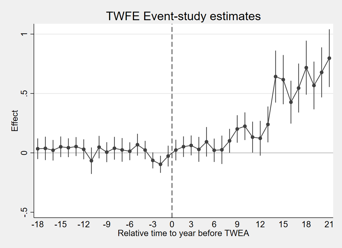
library(fixest); library(haven)
options(digits = 7)
load(url("https://raw.githubusercontent.com/Credible-Answers/did_book/main/cc_xd_didtextbook_2025_9_30/Data%20sets/Moser%20and%20Voena%202012/moser_voena_didtextbook.RData"))

reltimeminus_vars <- paste0("reltimeminus", 1:18)
reltimeplus_vars  <- paste0("reltimeplus", 1:21)
formula_str <- paste("patents ~", paste(reltimeminus_vars, collapse = " + "), "+",
                     paste(reltimeplus_vars, collapse = " + "), "+ treatmentgroup | year")
model4 <- feols(as.formula(formula_str), data = df, cluster = ~subclass)

rt <- c(-(18:1), 0, 1:21)
# 18:1 already gives the order -18,...,-1 (no rev())
coefs <- c(coef(model4)[paste0("reltimeminus", 18:1)], 0,
           coef(model4)[paste0("reltimeplus", 1:21)])
ses   <- c(se(model4)[paste0("reltimeminus", 18:1)], 0,
           se(model4)[paste0("reltimeplus", 1:21)])
png("figures/ch03_fig32_es_twfe_R.png", width = 1000, height = 600)
plot(rt, coefs, type = "b", pch = 19, col = "navy", cex = 0.6,
     xlab = "Relative time to year before TWEA", ylab = "Effect",
     main = "TWFE Event-study estimates",
     ylim = range(coefs - 1.96 * ses, coefs + 1.96 * ses))
# at rt = 0 the CI has zero length and arrows() warns: exclude that point
nz <- ses > 0
arrows(rt[nz], (coefs - 1.96 * ses)[nz], rt[nz], (coefs + 1.96 * ses)[nz],
       length = 0.03, angle = 90, code = 3, col = "firebrick")
abline(h = 0, col = "black", lwd = 0.8)
abline(v = 0, col = "black", lty = 2)
dev.off()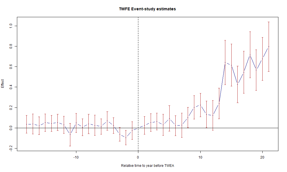
import pandas as pd
import pyfixest as pf
import matplotlib.pyplot as plt
import numpy as np

df = pd.read_parquet("https://raw.githubusercontent.com/Credible-Answers/did_book/main/cc_xd_didtextbook_2025_9_30/Data%20sets/Moser%20and%20Voena%202012/moser_voena_didtextbook.parquet")
minus_vars = [f"reltimeminus{i}" for i in range(1, 19)]
plus_vars = [f"reltimeplus{i}" for i in range(1, 22)]
fml = "patents ~ " + " + ".join(minus_vars + plus_vars) + " + treatmentgroup | year"
m4 = pf.feols(fml, data=df, vcov={'CRV1': 'subclass'})
rt = list(range(-18, 0)) + [0] + list(range(1, 22))
c4 = [m4.coef()[f"reltimeminus{i}"] for i in range(18, 0, -1)] + [0] + \
     [m4.coef()[f"reltimeplus{i}"] for i in range(1, 22)]
s4 = [m4.se()[f"reltimeminus{i}"] for i in range(18, 0, -1)] + [0] + \
     [m4.se()[f"reltimeplus{i}"] for i in range(1, 22)]
c4, s4 = np.array(c4), np.array(s4)
fig, ax = plt.subplots(figsize=(10, 6))
ax.plot(rt, c4, 'o-', color='navy', markersize=4, linewidth=1.2)
ax.errorbar(rt, c4, yerr=1.96*s4, fmt='none', ecolor='firebrick', capsize=2, linewidth=1)
ax.axhline(0, color='black', linewidth=0.8)
ax.axvline(0, color='black', linestyle='--', linewidth=0.8)
ax.set_xlabel("Relative time to year before TWEA")
ax.set_ylabel("Effect")
ax.set_title("TWFE Event-study estimates")
plt.tight_layout()
plt.savefig("figures/ch03_fig32_es_twfe_Python.png", dpi=150, bbox_inches="tight")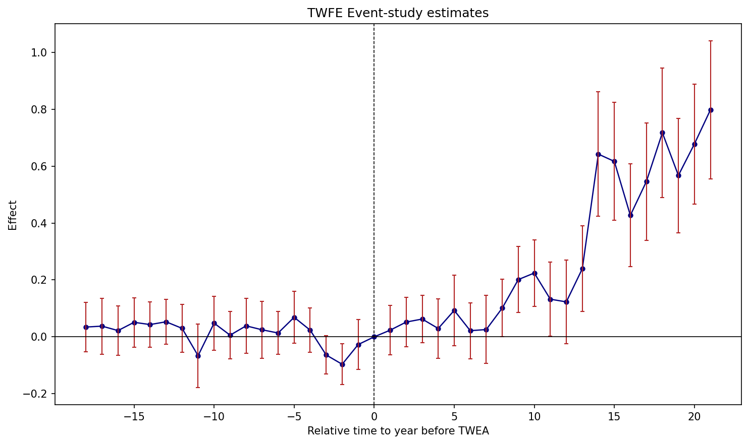
Figure 3.2: Effects of compulsory licensing on US innovation, according to an ES-TWFER. Standard errors clustered at the patent subclass level. 95% confidence intervals shown in red.
CQ#5: Effect of Compulsory Licensing
According to this regression, does compulsory licensing have an effect on US innovation?
Based on Figure 3.2.
Result: No short-term effect: the coefficients \(\hat\beta^{fe}_\ell\) are small and insignificant for \(\ell \in \{1,\dots,7\}\). After eight years, effects become positive and significant, and after 14 years they become very large.
CQ#6: Assumptions NA and PT
Do Assumptions NA and PT seem to hold?
Based on Figure 3.2, plus a joint test of the pre-trends (continues from CQ#4).
* F-test on pre-trends
test reltimeminus1 reltimeminus2 reltimeminus3 reltimeminus4 reltimeminus5 reltimeminus6 reltimeminus7 reltimeminus8 reltimeminus9 reltimeminus10 reltimeminus11 reltimeminus12 reltimeminus13 reltimeminus14 reltimeminus15 reltimeminus16 reltimeminus17 reltimeminus18
F( 18, 7247) = 3.79
Prob > F = 0.0000# F-test on pre-trends
linearHypothesis(model4, paste0("reltimeminus", 1:18))Chisq = 68.25, p-value = 8.915e-08# F-test on pre-trends
c = m4.coef()
v_mat = pd.DataFrame(m4._vcov, index=c.index, columns=c.index)
pre_names = [x for x in minus_vars if x in c.index]
beta_pre = c[pre_names].values
V_pre = v_mat.loc[pre_names, pre_names].values
F_stat = beta_pre @ np.linalg.inv(V_pre) @ beta_pre / len(pre_names)
p_val = 1 - stats.f.cdf(F_stat, len(pre_names), df["subclass"].nunique() - 1)
print(f"F-test: F({len(pre_names)}, {df['subclass'].nunique()-1}) = {F_stat:.4f}, p = {p_val:.4f}")F-test: F(18, 7247) = 3.7917, p = 0.0000Result: The pretrend estimates are small, and substantially smaller than the estimated mid- and long-run effects; only one out of 18 is individually significant at the 5% level. However, they are jointly significant (\(F = 3.79\), \(p < 0.001\)). The no-anticipation and parallel trends assumptions seem to hold in this application.
CQ#7: Verify Equation (3.7)
Verify that (3.7) holds for \(\ell = 1\), by computing in Stata the DID in the right hand side of that equation.
* Verify equation (3.7) for l=1 (continues from CQ#4)
quietly summarize patents if year==1919 & treatmentgroup==1
scalar m1 = r(mean)
quietly summarize patents if year==1918 & treatmentgroup==1
scalar m2 = r(mean)
quietly summarize patents if year==1919 & treatmentgroup==0
scalar m3 = r(mean)
quietly summarize patents if year==1918 & treatmentgroup==0
scalar m4 = r(mean)
display "DID manual = " m1-m2-(m3-m4)
DID manual (eq 3.7, l=1) = .02352017# DID manual (continues from CQ#4)
m1 <- mean(df$patents[df$year == 1919 & df$treatmentgroup == 1])
m2 <- mean(df$patents[df$year == 1918 & df$treatmentgroup == 1])
m3 <- mean(df$patents[df$year == 1919 & df$treatmentgroup == 0])
m4 <- mean(df$patents[df$year == 1918 & df$treatmentgroup == 0])
cat("DID manual:", m1 - m2 - (m3 - m4), "\n")
cat("reltimeplus1 coef:", coef(model4)["reltimeplus1"])DID manual (eq 3.7, l=1): 0.02352017
reltimeplus1 coef: 0.02352017# DID manual (continues from CQ#4)
m1v = df.loc[(df["year"]==1919) & (df["treatmentgroup"]==1), "patents"].mean()
m2v = df.loc[(df["year"]==1918) & (df["treatmentgroup"]==1), "patents"].mean()
m3v = df.loc[(df["year"]==1919) & (df["treatmentgroup"]==0), "patents"].mean()
m4v = df.loc[(df["year"]==1918) & (df["treatmentgroup"]==0), "patents"].mean()
print(f"DID manual (eq 3.7, l=1): {m1v - m2v - (m3v - m4v):.8f}")
print(f"reltimeplus1 coef: {m4.coef()['reltimeplus1']:.8f}")DID manual (eq 3.7, l=1): 0.02352017
reltimeplus1 coef: 0.02352017Result: The manual DID (0.02352) matches reltimeplus1 exactly.
CQ#8: Linear Pre-Trends We Could Fail to Detect
Use the pretrends package (Roth, 2022) to compute the linear differential trends one has 50% chances of detecting based on the first 6 pre-trend estimators.
* ssc install pretrends, replace
copy "https://raw.githubusercontent.com/Credible-Answers/did_book/main/cc_xd_didtextbook_2025_9_30/Data%20sets/Moser%20and%20Voena%202012/moser_voena_didtextbook.dta" "moser_voena_didtextbook.dta", replace
use "moser_voena_didtextbook.dta", clear
forvalues l = 1/18 {
    cap gen reltimeminus`l' = treatmentgroup * (year == 1918 - `l')
}
forvalues l = 1/21 {
    cap gen reltimeplus`l' = treatmentgroup * (year == 1918 + `l')
}
reghdfe patents reltimeminus* reltimeplus*, absorb(treatmentgroup year) cluster(subclass)
pretrends power 0.5, numpre(6)
Slope for 50% power = .0098235library(haven); library(fixest); library(pretrends)
load(url("https://raw.githubusercontent.com/Credible-Answers/did_book/main/cc_xd_didtextbook_2025_9_30/Data%20sets/Moser%20and%20Voena%202012/moser_voena_didtextbook.RData"))
for (l in 1:18) df[[paste0("reltimeminus", l)]] <- as.numeric(df$treatmentgroup == 1 & df$year == 1918 - l)
for (l in 1:21) df[[paste0("reltimeplus", l)]] <- as.numeric(df$treatmentgroup == 1 & df$year == 1918 + l)
model6 <- feols(as.formula(paste(
"patents ~", paste(paste0("reltimeminus", 1:18), collapse = " + "), "+",
paste(paste0("reltimeplus", 1:21), collapse = " + "), "| treatmentgroup + year")),
data = df, cluster = ~subclass)
# Extract coefficients and vcov for first 6 pre-periods
pretrend_coefs_6 <- paste0("reltimeminus", 1:6)
beta <- coef(model6)[pretrend_coefs_6]
sigma <- vcov(model6)[pretrend_coefs_6, pretrend_coefs_6]
slope50 <- slope_for_power(sigma = sigma, targetPower = 0.5,
tVec = -6:-1, referencePeriod = 0)
cat("Slope for 50% power:", slope50)Slope for 50% power (numpre=6): 0.009796021import pandas as pd
import pyfixest as pf
from pretrends import slope_for_power
df = pd.read_parquet("https://raw.githubusercontent.com/Credible-Answers/did_book/main/cc_xd_didtextbook_2025_9_30/Data%20sets/Moser%20and%20Voena%202012/moser_voena_didtextbook.parquet")
for l in range(1, 19):
df[f"reltimeminus{l}"] = (df["treatmentgroup"] * (df["year"] == 1918 - l)).astype(float)
for l in range(1, 22):
df[f"reltimeplus{l}"] = (df["treatmentgroup"] * (df["year"] == 1918 + l)).astype(float)
minus_vars = [f"reltimeminus{i}" for i in range(1, 19)]
plus_vars = [f"reltimeplus{i}" for i in range(1, 22)]
# Full model (matches Stata: reghdfe patents reltimeminus* reltimeplus*)
fml6 = "patents ~ " + " + ".join(minus_vars + plus_vars) + " | treatmentgroup + year"
m6 = pf.feols(fml6, data=df, vcov={"CRV1": "subclass"})
# Extract vcov for 6 closest pre-periods
pre6 = [f"reltimeminus{i}" for i in range(1, 7)]
vcov6 = pd.DataFrame(m6._vcov, index=m6.coef().index,
columns=m6.coef().index).loc[pre6, pre6].values
slope50 = slope_for_power(vcov6, target_power=0.5,
t_vec=[-6, -5, -4, -3, -2, -1])
print(f"Slope for 50% power (numpre=6): {slope50:.7f}")Slope for 50% power (numpre=6): 0.0098252Note: All three platforms give essentially identical results: Stata ≈ 0.0098235, R ≈ 0.009796, Python ≈ 0.0098252. The Python pretrends package (based on Roth 2022) uses the exact multivariate normal CDF, matching Stata and R.
CQ#9: Event-Study without Pre-Trends
Using the
moser_voena_didtextbookdataset, estimate the ES-TWFER in (3.22) with patents as the outcome. Are the estimated effects of compulsory licensing in this regression similar to those we obtained estimating (3.7)? Are the effects more precisely estimated?
copy "https://raw.githubusercontent.com/Credible-Answers/did_book/main/cc_xd_didtextbook_2025_9_30/Data%20sets/Moser%20and%20Voena%202012/moser_voena_didtextbook.dta" "moser_voena_didtextbook.dta", replace
use "moser_voena_didtextbook.dta", clear
forvalues l = 1/21 {
    cap gen reltimeplus`l' = treatmentgroup * (year == 1918 + `l')
}
reg patents i.yearpost treatmentgroup reltimeplus*, cluster(subclass)
(Std. err. adjusted for 7,248 clusters in subclass)
--------------------------------------------------------------------------------
| Robust
patents | Coefficient std. err. t P>|t| [95% conf. interval]
---------------+----------------------------------------------------------------
treatmentgroup | -.1780874 .0338176 -5.27 0.000 -.2443797 -.1117951
reltimeplus1 | .0108007 .0309763 0.35 0.727 -.049922 .0715233
reltimeplus2 | .0393018 .0302047 1.30 0.193 -.0199081 .0985118
reltimeplus3 | .0498425 .0359726 1.39 0.166 -.0206743 .1203593
reltimeplus4 | .0166497 .0418098 0.40 0.690 -.0653098 .0986092
reltimeplus5 | .0803071 .049547 1.62 0.105 -.0168195 .1774337
reltimeplus6 | .0089819 .041055 0.22 0.827 -.0714978 .0894616
reltimeplus7 | .0129501 .0472633 0.27 0.784 -.0796997 .1056
reltimeplus8 | .0885536 .0432021 2.05 0.040 .0038648 .1732424
reltimeplus9 | .1885454 .0479442 3.93 0.000 .0945607 .28253
reltimeplus10 | .2115488 .050361 4.20 0.000 .1128266 .310271
reltimeplus11 | .1196796 .0520212 2.30 0.021 .017703 .2216563
reltimeplus12 | .1101517 .0593023 1.86 0.063 -.0060982 .2264015
reltimeplus13 | .2266778 .0691283 3.28 0.001 .0911663 .3621893
reltimeplus14 | .6294969 .1040565 6.05 0.000 .4255158 .833478
reltimeplus15 | .6038686 .0994844 6.07 0.000 .4088502 .798887
reltimeplus16 | .4141158 .0858483 4.82 0.000 .2458282 .5824034
reltimeplus17 | .5330394 .0957086 5.57 0.000 .3454227 .7206561
reltimeplus18 | .7046044 .109204 6.45 0.000 .4905328 .918676
reltimeplus19 | .5546581 .0930222 5.96 0.000 .3723075 .7370087
reltimeplus20 | .6650045 .1024705 6.49 0.000 .4641324 .8658766
reltimeplus21 | .7847135 .1190138 6.59 0.000 .5514119 1.018015
_cons | .3143656 .0098193 32.02 0.000 .2951169 .3336142
--------------------------------------------------------------------------------library(haven); library(fixest)
load(url("https://raw.githubusercontent.com/Credible-Answers/did_book/main/cc_xd_didtextbook_2025_9_30/Data%20sets/Moser%20and%20Voena%202012/moser_voena_didtextbook.RData"))
for (l in 1:21) df[[paste0("reltimeplus", l)]] <- as.numeric(df$treatmentgroup == 1 & df$year == 1918 + l)
post_formula <- as.formula(paste(
"patents ~ i(yearpost) + treatmentgroup +",
paste(paste0("reltimeplus", 1:21), collapse = " + ")))
model5 <- feols(post_formula, data = df, cluster = ~subclass)
summary(model5) Estimate Std. Error t value Pr(>|t|)
treatmentgroup -0.178087 0.033818 -5.266118 1.4334e-07 ***
reltimeplus1 0.010801 0.030976 0.348674 7.2734e-01
reltimeplus2 0.039302 0.030205 1.301183 1.9324e-01
reltimeplus3 0.049843 0.035973 1.385634 1.6590e-01
reltimeplus4 0.016650 0.041810 0.398234 6.9050e-01
reltimeplus5 0.080307 0.049547 1.620753 1.0514e-01
reltimeplus6 0.008982 0.041055 0.218776 8.2685e-01
reltimeplus7 0.012950 0.047263 0.274032 7.8404e-01
reltimeplus8 0.088554 0.043202 2.049798 4.0405e-02 *
reltimeplus9 0.188545 0.047944 3.932590 8.4570e-05 ***
reltimeplus10 0.211549 0.050361 4.201191 2.6755e-05 ***
reltimeplus11 0.119680 0.052021 2.300631 2.1441e-02 *
reltimeplus12 0.110152 0.059302 1.857479 6.3256e-02
reltimeplus13 0.226678 0.069128 3.278641 1.0478e-03 **
reltimeplus14 0.629497 0.104057 6.050261 1.5073e-09 ***
reltimeplus15 0.603869 0.099484 6.069422 1.3510e-09 ***
reltimeplus16 0.414116 0.085848 4.823560 1.4305e-06 ***
reltimeplus17 0.533039 0.095709 5.568517 2.6464e-08 ***
reltimeplus18 0.704604 0.109204 6.452210 1.1588e-10 ***
reltimeplus19 0.554658 0.093022 5.963752 2.5802e-09 ***
reltimeplus20 0.665005 0.102471 6.490150 9.2071e-11 ***
reltimeplus21 0.784714 0.119014 6.593469 4.5985e-11 ***
---
RMSE: 1.33696 Adj. R2: 0.025481import pandas as pd
import pyfixest as pf
df = pd.read_parquet("https://raw.githubusercontent.com/Credible-Answers/did_book/main/cc_xd_didtextbook_2025_9_30/Data%20sets/Moser%20and%20Voena%202012/moser_voena_didtextbook.parquet")
for l in range(1, 22):
df[f"reltimeplus{l}"] = (df["treatmentgroup"] * (df["year"] == 1918 + l)).astype(float)
plus_vars = [f"reltimeplus{i}" for i in range(1, 22)]
fml5 = "patents ~ " + " + ".join(plus_vars) + " + treatmentgroup | yearpost"
m5 = pf.feols(fml5, data=df, vcov={"CRV1": "subclass"})
print(m5.summary())| Coefficient | Estimate | Std. Error | t value | Pr(>|t|) | 2.5% | 97.5% |
|:---------------|------------|--------------|-----------|------------|---------|---------|
| reltimeplus1 | 0.01080 | 0.03098 | 0.34867 | 0.72734 | -0.0499 | 0.072 |
| reltimeplus2 | 0.03930 | 0.03020 | 1.30118 | 0.19324 | -0.0199 | 0.099 |
| reltimeplus3 | 0.04984 | 0.03597 | 1.38563 | 0.16590 | -0.0207 | 0.120 |
| reltimeplus4 | 0.01665 | 0.04181 | 0.39823 | 0.69050 | -0.0653 | 0.099 |
| reltimeplus5 | 0.08031 | 0.04955 | 1.62075 | 0.10514 | -0.0168 | 0.177 |
| reltimeplus6 | 0.00898 | 0.04106 | 0.21878 | 0.82685 | -0.0715 | 0.089 |
| reltimeplus7 | 0.01295 | 0.04726 | 0.27403 | 0.78404 | -0.0797 | 0.106 |
| reltimeplus8 | 0.08855 | 0.04320 | 2.04980 | 0.04041 | 0.0039 | 0.173 |
| reltimeplus9 | 0.18855 | 0.04794 | 3.93259 | 0.00008 | 0.0946 | 0.283 |
| reltimeplus10 | 0.21155 | 0.05036 | 4.20119 | 0.00003 | 0.1128 | 0.310 |
| reltimeplus11 | 0.11968 | 0.05202 | 2.30063 | 0.02144 | 0.0177 | 0.222 |
| reltimeplus12 | 0.11015 | 0.05930 | 1.85748 | 0.06326 | -0.0061 | 0.226 |
| reltimeplus13 | 0.22668 | 0.06913 | 3.27864 | 0.00105 | 0.0912 | 0.362 |
| reltimeplus14 | 0.62950 | 0.10406 | 6.05026 | 0.00000 | 0.4255 | 0.833 |
| reltimeplus15 | 0.60387 | 0.09948 | 6.06942 | 0.00000 | 0.4089 | 0.799 |
| reltimeplus16 | 0.41412 | 0.08585 | 4.82356 | 0.00000 | 0.2458 | 0.582 |
| reltimeplus17 | 0.53304 | 0.09571 | 5.56852 | 0.00000 | 0.3454 | 0.721 |
| reltimeplus18 | 0.70460 | 0.10920 | 6.45221 | 0.00000 | 0.4905 | 0.919 |
| reltimeplus19 | 0.55466 | 0.09302 | 5.96375 | 0.00000 | 0.3723 | 0.737 |
| reltimeplus20 | 0.66500 | 0.10247 | 6.49015 | 0.00000 | 0.4641 | 0.866 |
| reltimeplus21 | 0.78471 | 0.11901 | 6.59347 | 0.00000 | 0.5514 | 1.018 |
| treatmentgroup | -0.17809 | 0.03382 | -5.26612 | 0.00000 | -0.2444 | -0.112 |
---
RMSE: 1.337 R2: 0.026 R2 Within: 0.001Figure 3.5: Comparison of two ES-TWFER estimators
copy "https://raw.githubusercontent.com/Credible-Answers/did_book/main/cc_xd_didtextbook_2025_9_30/Data%20sets/Moser%20and%20Voena%202012/moser_voena_didtextbook.dta" "moser_voena_didtextbook.dta", replace
use "moser_voena_didtextbook.dta", clear

reg patents i.year treatmentgroup reltimeminus* reltimeplus*, cluster(subclass)
estimates store m1

reg patents i.yearpost treatmentgroup reltimeplus*, cluster(subclass)
estimates store m2

coefplot (m1, label("With Pre-Periods") mcolor(gs10) ciopts(lcolor(gs10)) connect(l) lcolor(gs10) msymbol(O) msize(small)) ///
         (m2, label("Without Pre-Periods") mcolor(gs4) ciopts(lcolor(gs4)) connect(l) lcolor(gs4) msymbol(O) msize(small)), ///
    keep(reltimeplus*) vertical ///
    yline(0, lcolor(gs12) lpattern(solid)) ///
    title("TWFE Event-study estimates") ///
    xtitle("Relative time to year before TWEA") ///
    ytitle("Effect") ///
    legend(rows(1) position(6)) ///
    scheme(s2mono) ///
    xlabel(1 "0" 4 "3" 7 "6" 10 "9" 13 "12" 16 "15" 19 "18" 21 "21", noticks)
graph export "figures/ch03_fig35_comparison.png", replace width(1200)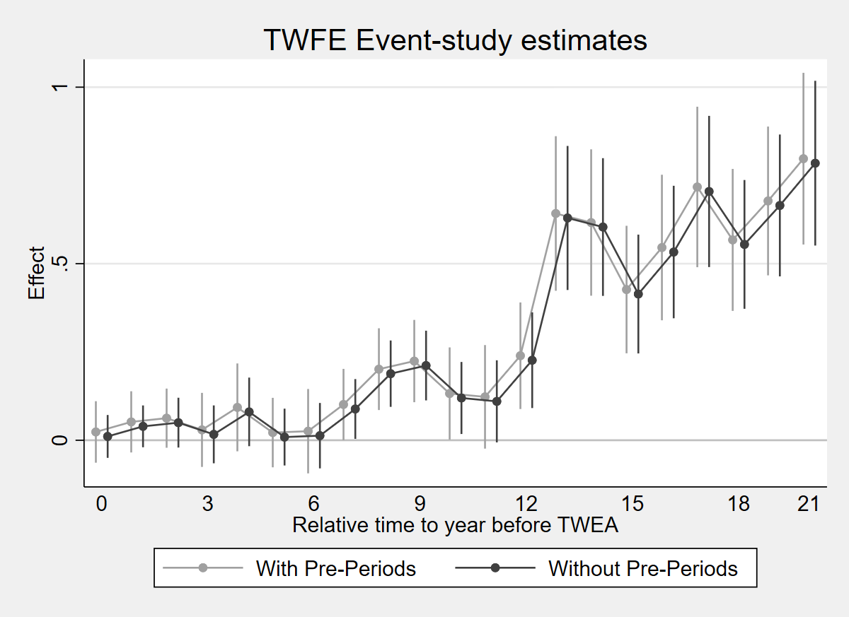
library(fixest); library(dplyr); library(ggplot2)
load(url("https://raw.githubusercontent.com/Credible-Answers/did_book/main/cc_xd_didtextbook_2025_9_30/Data%20sets/Moser%20and%20Voena%202012/moser_voena_didtextbook.RData"))

reltimeminus_vars <- paste0("reltimeminus", 1:18)
reltimeplus_vars <- paste0("reltimeplus", 1:21)

fml1 <- as.formula(paste("patents ~ i(year) + treatmentgroup +", paste(c(reltimeminus_vars, reltimeplus_vars), collapse = " + ")))
m1 <- feols(fml1, data = df, cluster = ~subclass)

fml2 <- as.formula(paste("patents ~ i(yearpost) + treatmentgroup +", paste(reltimeplus_vars, collapse = " + ")))
m2 <- feols(fml2, data = df, cluster = ~subclass)

coef1 <- data.frame(x = 1:21, est = coef(m1)[reltimeplus_vars], se = se(m1)[reltimeplus_vars], model = "With Pre-Periods")
coef2 <- data.frame(x = 1:21, est = coef(m2)[reltimeplus_vars], se = se(m2)[reltimeplus_vars], model = "Without Pre-Periods")
plotdf <- rbind(coef1, coef2)
plotdf$lo <- plotdf$est - 1.96 * plotdf$se
plotdf$hi <- plotdf$est + 1.96 * plotdf$se

ggplot(plotdf, aes(x = x, y = est, color = model)) +
  geom_line(position = position_dodge(0.3)) +
  geom_point(position = position_dodge(0.3), size = 1.5) +
  geom_errorbar(aes(ymin = lo, ymax = hi), width = 0.3, position = position_dodge(0.3)) +
  geom_hline(yintercept = 0, linetype = "solid", color = "grey70") +
  scale_color_manual(values = c("With Pre-Periods" = "grey70", "Without Pre-Periods" = "grey30")) +
  scale_x_continuous(breaks = c(1, 4, 7, 10, 13, 16, 19, 21), labels = c("0", "3", "6", "9", "12", "15", "18", "21")) +
  labs(x = "Relative time to year before TWEA", y = "Effect", title = "TWFE Event-study estimates", color = "") +
  theme_minimal() + theme(legend.position = "bottom")
ggsave("figures/ch03_fig35_comparison_R.png", width = 8, height = 5, dpi = 150)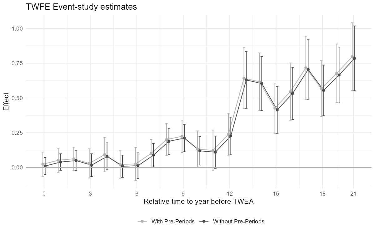
import pandas as pd
import numpy as np
import pyfixest as pf
import matplotlib.pyplot as plt

df = pd.read_parquet("https://raw.githubusercontent.com/Credible-Answers/did_book/main/cc_xd_didtextbook_2025_9_30/Data%20sets/Moser%20and%20Voena%202012/moser_voena_didtextbook.parquet")

minus_vars = [f"reltimeminus{i}" for i in range(1, 19)]
plus_vars = [f"reltimeplus{i}" for i in range(1, 22)]

fml1 = "patents ~ " + " + ".join(minus_vars + plus_vars) + " + C(year) + treatmentgroup"
m1 = pf.feols(fml1, data=df, vcov={"CRV1": "subclass"})

fml2 = "patents ~ " + " + ".join(plus_vars) + " + C(yearpost) + treatmentgroup"
m2 = pf.feols(fml2, data=df, vcov={"CRV1": "subclass"})

x = np.arange(1, 22)
c1 = np.array([m1.coef()[v] for v in plus_vars])
s1 = np.array([m1.se()[v] for v in plus_vars])
c2 = np.array([m2.coef()[v] for v in plus_vars])
s2 = np.array([m2.se()[v] for v in plus_vars])

fig, ax = plt.subplots(figsize=(8, 5))
ax.errorbar(x - 0.1, c1, yerr=1.96*s1, fmt='-o', color='grey', markersize=3, linewidth=1, capsize=2, capthick=0.8, elinewidth=0.8, label='With Pre-Periods')
ax.errorbar(x + 0.1, c2, yerr=1.96*s2, fmt='-o', color='black', markersize=3, linewidth=1, capsize=2, capthick=0.8, elinewidth=0.8, label='Without Pre-Periods')
ax.axhline(y=0, color='grey', linestyle='-', linewidth=0.5)
ax.set_xticks([1, 4, 7, 10, 13, 16, 19, 21])
ax.set_xticklabels(["0", "3", "6", "9", "12", "15", "18", "21"])
ax.set_xlabel("Relative time to year before TWEA")
ax.set_ylabel("Effect")
ax.set_title("TWFE Event-study estimates")
ax.legend(loc='upper left', frameon=False)
ax.set_ylim(-0.25, 1.1)
plt.tight_layout()
plt.savefig("figures/ch03_fig35_comparison_Python.png", dpi=150)
plt.show()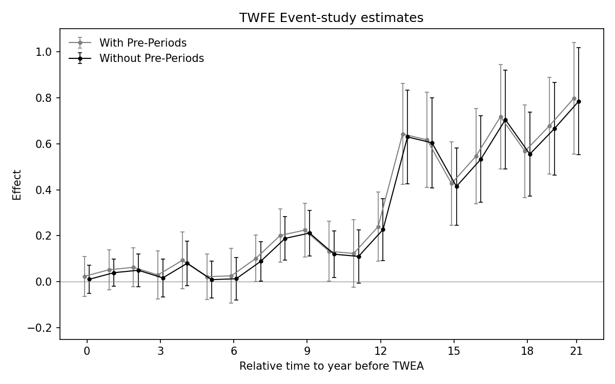
Figure 3.5: Effects of compulsory licensing on US innovation: comparison of two ES-TWFER estimators. The coefficients shown in grey come from the usual ES-TWFER with FEs for pre-treatment periods. The coefficients shown in black come from the imputation ES-TWFER without FEs for pre-treatment periods. Standard errors are clustered at the patent subclass level. 95% confidence intervals shown.
CQ#10: Variance of Treatment Effects
Compare the variance of
diffpatentswrt1918in treatment and control groups in 1932.
copy "https://raw.githubusercontent.com/Credible-Answers/did_book/main/cc_xd_didtextbook_2025_9_30/Data%20sets/Moser%20and%20Voena%202012/moser_voena_didtextbook.dta" "moser_voena_didtextbook.dta", replace
use "moser_voena_didtextbook.dta", clear
sdtest diffpatentswrt1918 if year==1932, by(treatmentgroup)

scalar sd_effects = r(sd_2) - r(sd_1)
reg diffpatentswrt1918 treatmentgroup if year==1932
display "Bottom and top decile of effects: [" _b[treatmentgroup] - 1.28*sd_effects ", " _b[treatmentgroup] + 1.28*sd_effects "]
Variance ratio test
------------------------------------------------------------------------------
   Group |     Obs        Mean    Std. err.   Std. dev.   [95% conf. interval]
---------+--------------------------------------------------------------------
       0 |   6,912    .3577836    .0213236    1.772807    .3159828    .3995843
       1 |     336           1    .1097584    2.011905    .7840975    1.215903
---------+--------------------------------------------------------------------
Combined |   7,248    .3875552    .0210201    1.789547    .3463497    .4287606
------------------------------------------------------------------------------

    ratio = sd(0) / sd(1)                        f =   0.7764
  Pr(F < f) = 0.0004     2*Pr(F < f) = 0.0008

sd_2 - sd_1 = .23909779
beta = .64221644
Bottom and top decile of effects: [.33617126, .94826161]library(haven)
library(dplyr)
load(url("https://raw.githubusercontent.com/Credible-Answers/did_book/main/cc_xd_didtextbook_2025_9_30/Data%20sets/Moser%20and%20Voena%202012/moser_voena_didtextbook.RData"))
df_1932 <- df %>% filter(year == 1932)
var_test <- var.test(diffpatentswrt1918 ~ treatmentgroup, data = df_1932)
print(var_test)
sd_stats <- df_1932 %>%
group_by(treatmentgroup) %>%
summarise(sd = sd(diffpatentswrt1918, na.rm = TRUE))
sd_effects <- sd_stats$sd[2] - sd_stats$sd[1]
effect_reg <- lm(diffpatentswrt1918 ~ treatmentgroup, data = df_1932)
beta_reg <- coef(effect_reg)["treatmentgroup"]
cat(
"Bottom and top decile of effects: [",
beta_reg - 1.28 * sd_effects,
",",
beta_reg + 1.28 * sd_effects,
"]\n"
)F = 0.77644, p-value = 0.0008145
SD control: 1.772807
SD treated: 2.011905
sd_2 - sd_1 = 0.2390978
beta = 0.6422164
Bottom and top decile of effects: [ 0.3361713 , 0.9482616 ]import pandas as pd
import pyfixest as pf
from scipy import stats
df = pd.read_parquet(
"https://raw.githubusercontent.com/Credible-Answers/did_book/main/cc_xd_didtextbook_2025_9_30/Data%20sets/Moser%20and%20Voena%202012/moser_voena_didtextbook.parquet"
)
df_1932 = df[df["year"] == 1932]
g0 = df_1932.loc[
df_1932["treatmentgroup"] == 0,
"diffpatentswrt1918"
].dropna()
g1 = df_1932.loc[
df_1932["treatmentgroup"] == 1,
"diffpatentswrt1918"
].dropna()
sd0 = g0.std(ddof=1)
sd1 = g1.std(ddof=1)
sd_effects = sd1 - sd0
F_var = sd0**2 / sd1**2
p_two = 2 * min(
stats.f.cdf(F_var, len(g0) - 1, len(g1) - 1),
1 - stats.f.cdf(F_var, len(g0) - 1, len(g1) - 1)
)
m7 = pf.feols(
"diffpatentswrt1918 ~ treatmentgroup",
data=df_1932
)
beta = m7.coef()["treatmentgroup"]
print(f"F = {F_var:.4f}, p = {p_two:.4f}")
print(f"sd_2 - sd_1 = {sd_effects:.6f}")
print(f"beta = {beta:.6f}")
print(
f"Bottom and top decile of effects: "
f"[{beta - 1.28 * sd_effects:.6f}, "
f"{beta + 1.28 * sd_effects:.6f}]"
)F = 0.7765, p = 0.0008
sd_2 - sd_1 = 0.238982
beta = 0.642216
Bottom and top decile of effects: [0.336320, 0.948113]Result: The treated group has a larger variance (\(\hat{\sigma}_1 = 2.01 > \hat{\sigma}_0 = 1.77\)). The implied SD of treatment effects is \(\approx 0.239\), and the bottom and top deciles of subclass-specific effects are respectively equal to 0.336 and 0.948. version 2909