Chapter 8: Staggered first switch designs
Overview
Dataset: Gentzkow, Shapiro & Sinkinson (2011) — gentzkowetal_didtextbook.dta (Stata), gentzkowetal_didtextbook.RData (R), gentzkowetal_didtextbook.parquet (Python) (16,872 observations, 1,195 counties, 16 election years 1868–1928)
This chapter studies staggered first switch designs where groups experience their first treatment change at different points in time. These designs nest staggered adoption designs. But staggered first switch designs also encompass more general designs, where the treatment may be nonbinary and/or non-absorbing. The running example measures the effect of the number of daily newspapers (numdailies) on presidential voter turnout (prestout).
Key topics: static TWFE decompositions with multiple treatments (twowayfeweights), non-normalized and normalized event-study estimators (did_multiplegt_dyn), treatment-path descriptions (design option), and heterogeneity-robust estimators ruling out dynamic effects (did_multiplegt_stat).
7 computer questions + 2 Figures.
Packages used:
| Task | Stata | R | Python |
|---|---|---|---|
| OLS / TWFE | reg, areg |
fixest, sandwich |
pyfixest |
| Weight decomposition | twowayfeweights (SSC) |
TwoWayFEWeights (CRAN) |
twowayfeweights |
| Event-study DID | did_multiplegt_dyn (SSC) |
DIDmultiplegtDYN (CRAN) |
py-did-multiplegt-dyn (PyPI) |
| Static DID (ATS/WATS) | did_multiplegt_stat (SSC) |
DIDmultiplegtSTAT (GitHub) |
py_did_multiplegt_stat (PyPI) |
Installation notes:
- R
DIDmultiplegtSTAT:devtools::install_github("chaisemartinPackages/did_multiplegt_stat/R", force = TRUE) - R
DIDmultiplegtDYN: Thedesign()option works withdesign=c(0.8,"console"). Effects match across platforms. - Python
did_multiplegt_dyn:pip install py-did-multiplegt-dyn. RequirespolarsDataFrames. - Python
did_multiplegt_stat: Local notebook-based translation; seepy_did_multiplegt_stat.
Note on cross-platform differences: CQ41–CQ43 match exactly between Stata and R to 7 decimals. CQ49 (did_multiplegt_stat) shows small differences between Stata and Python due to internal implementation variations. N, switchers, and stayers counts are identical across all three.
CQ#40: Distributed-Lag TWFE Regression
Regress turnout on the number of newspapers and its lag, with county and year FEs, clustering standard errors at the county level. Interpret the results.
copy "https://raw.githubusercontent.com/Credible-Answers/did_book/main/cc_xd_didtextbook_2025_9_30/Data%20sets/Gentzkow%20et%20al%202011/gentzkowetal_didtextbook.dta" "gentzkowetal_didtextbook.dta", replace
use "gentzkowetal_didtextbook.dta", clear
reghdfe prestout i.year numdailies lag_numdailies, absorb(cnty90) cluster(cnty90)
(Std. err. adjusted for 1,195 clusters in cnty90)
--------------------------------------------------------------------------------
| Robust
prestout | Coefficient std. err. t P>|t| [95% conf. interval]
----------------+----------------------------------------------------------------
numdailies | -.0007962 .0013856 -0.57 0.566 -.0035147 .0019224
lag_numdailies | .0050348 .0014465 3.48 0.001 .0021968 .0078728
--------------------------------------------------------------------------------
N = 15,629library(haven); library(fixest)
load(url("https://raw.githubusercontent.com/Credible-Answers/did_book/main/cc_xd_didtextbook_2025_9_30/Data%20sets/Gentzkow%20et%20al%202011/gentzkowetal_didtextbook.RData"))
gq3b <- feols(prestout ~ numdailies + lag_numdailies | cnty90 + year,
data = df, cluster = ~cnty90)
summary(gq3b) Estimate Std. Error t value Pr(>|t|)
numdailies -0.0007962 0.0013856 -0.5746 0.5657
lag_numdailies 0.0050348 0.0014465 3.4807 0.0005
N = 15,629import pandas as pd
import pyfixest as pf
df = pd.read_parquet("https://raw.githubusercontent.com/Credible-Answers/did_book/main/cc_xd_didtextbook_2025_9_30/Data%20sets/Gentzkow%20et%20al%202011/gentzkowetal_didtextbook.parquet")
m8 = pf.feols("prestout ~ numdailies + lag_numdailies + C(year) | cnty90", data=df, vcov={"CRV1": "cnty90"}, ssc=pf.ssc(adj=True, fixef_k="nonnested", cluster_adj=True))
print(m8.summary())| Coefficient | Estimate | Std. Error | t value | Pr(>|t|) | 2.5% | 97.5% |
|:----------------|-----------:|-------------:|------------:|-----------:|-----------:|-----------:|
| numdailies | -0.0007962 | 0.0013856 | -0.5745820 | 0.5656823 | -0.0035147 | 0.0019224 |
| lag_numdailies | 0.0050348 | 0.0014465 | 3.4806732 | 0.0005182 | 0.0021968 | 0.0078728 |
N = 15,629Interpretation: The distributed-lag TWFE regression gives \(\hat\beta_0^{dl} = -0.0007962\) (insignificant) and \(\hat\beta_1^{dl} = 0.0050348\) (significant). The contemporaneous effect of newspapers on turnout is small and insignificant, while the lagged effect is positive and significant.
CQ#41: Weight Decomposition (twowayfeweights)
Use the
twowayfeweightscommand and theother_treatmentsoption to decompose \(\hat\beta_0^{dl}\) and \(\hat\beta_1^{dl}\), and interpret the results.
copy "https://raw.githubusercontent.com/Credible-Answers/did_book/main/cc_xd_didtextbook_2025_9_30/Data%20sets/Gentzkow%20et%20al%202011/gentzkowetal_didtextbook.dta" "gentzkowetal_didtextbook.dta", replace
use "gentzkowetal_didtextbook.dta", clear
twowayfeweights prestout cnty90 year numdailies, other_treatments(lag_numdailies) type(feTR)
twowayfeweights prestout cnty90 year lag_numdailies, other_treatments(numdailies) type(feTR)
--- Decomposition of beta on numdailies (β = -0.0008) ---
Under the common trends assumption, beta estimates a weighted sum of 10,056 ATTs.
------------------------------------------------
Treat. var: numdailies # ATTs Σ weights
------------------------------------------------
Positive weights 5754 1.8541
Negative weights 4302 -0.8541
------------------------------------------------
Total 10056 1.0000
------------------------------------------------
Other treatment (lag_numdailies):
------------------------------------------------
Other treat.: lag_numd~s# ATTs Σ weights
------------------------------------------------
Positive weights 4721 1.2137
Negative weights 4618 -1.2137
------------------------------------------------
Total 9339 0.0000
------------------------------------------------
--- Decomposition of beta on lag_numdailies (β = 0.0050) ---
Under the common trends assumption, beta estimates a weighted sum of 9,339 ATTs.
------------------------------------------------
Treat. var: lag_numdai~s# ATTs Σ weights
------------------------------------------------
Positive weights 5273 1.7820
Negative weights 4066 -0.7820
------------------------------------------------
Total 9339 1.0000
------------------------------------------------
Other treatment (numdailies):
------------------------------------------------
Other treat.: numdailies# ATTs Σ weights
------------------------------------------------
Positive weights 4933 1.3558
Negative weights 5123 -1.3558
------------------------------------------------
Total 10056 0.0000
------------------------------------------------library(haven); library(TwoWayFEWeights)
load(url("https://raw.githubusercontent.com/Credible-Answers/did_book/main/cc_xd_didtextbook_2025_9_30/Data%20sets/Gentzkow%20et%20al%202011/gentzkowetal_didtextbook.RData"))
gq3a <- twowayfeweights(df, "prestout", "cnty90", "year", "numdailies", type = "feTR", other_treatments = "lag_numdailies")
gq3b <- twowayfeweights(df, "prestout", "cnty90", "year", "lag_numdailies", type = "feTR", other_treatments = "numdailies")--- Decomposition of beta on numdailies (β = -0.0008) ---
Σ positive weights = 1.8541 (5,754 ATTs)
Σ negastive weights = -0.8541 (4,302 ATTs)
Other treatment: 4,721 pos (Σ = 1.2137) | 4,618 neg (Σ = -1.2137)
--- Decomposition of beta on lag_numdailies (β = 0.0050) ---
Σ positive weights = 1.7820 (5,273 ATTs)
Σ negative weights = -0.7820 (4,066 ATTs)
Other treatment: 4,933 pos (Σ = 1.3558) | 5,123 neg (Σ = -1.3558)import pandas as pd
from twowayfeweights import twowayfeweights
df = pd.read_parquet("https://raw.githubusercontent.com/Credible-Answers/did_book/main/cc_xd_didtextbook_2025_9_30/Data%20sets/Gentzkow%20et%20al%202011/gentzkowetal_didtextbook.parquet")
res_a = twowayfeweights(df, "prestout", "cnty90", "year", "numdailies", type="feTR", other_treatments="lag_numdailies")
res_b = twowayfeweights(df, "prestout", "cnty90", "year", "lag_numdailies", type="feTR", other_treatments="numdailies")Under the common trends assumption,
the TWFE coefficient beta, equal to -0.0008, estimates the sum of several terms.
The first term is a weighted sum of 10056 ATTs of the treatment.
5754 ATTs receive a positive weight, and 4302 receive a negative weight.
------------------------------------------------
Treat. var: numdailies # ATTs Σ weights
------------------------------------------------
Positive weights 5754 1.8541
Negative weights 4302 -0.8541
------------------------------------------------
Total 10056 1.0000
------------------------------------------------
The next term is a weighted sum of 9339 ATTs of treatment 1 included in the other_treatments option.
4721 ATTs receive a positive weight, and 4618 receive a negative weight.
------------------------------------------------------
Other treat.: lag_numdailies # ATTs Σ weights
------------------------------------------------------
Positive weights 4721 1.2137
Negative weights 4618 -1.2137
------------------------------------------------------
Total 9339 0.0000
------------------------------------------------------
The development of this package was funded by the European Union (ERC, REALLYCREDIBLE,GA N°101043899).
Under the common trends assumption,
the TWFE coefficient beta, equal to 0.0050, estimates the sum of several terms.
The first term is a weighted sum of 9339 ATTs of the treatment.
5273 ATTs receive a positive weight, and 4066 receive a negative weight.
----------------------------------------------------
Treat. var: lag_numdailies # ATTs Σ weights
----------------------------------------------------
Positive weights 5273 1.7820
Negative weights 4066 -0.7820
----------------------------------------------------
Total 9339 1.0000
----------------------------------------------------
The next term is a weighted sum of 10056 ATTs of treatment 1 included in the other_treatments option.
4933 ATTs receive a positive weight, and 5123 receive a negative weight.
--------------------------------------------------
Other treat.: numdailies # ATTs Σ weights
--------------------------------------------------
Positive weights 4933 1.3558
Negative weights 5123 -1.3558
--------------------------------------------------
Total 10056 0.0000
--------------------------------------------------
Interpretation: \(\hat\beta^{dl}_0\) estimates the sum of two terms. The first term is a weighted combination of 10 056 \((g,t)\)-specific effects of current newspapers, where 5754 effects receive a positive weight, 4302 receive a negative weight, and where positive (resp. negative) weights sum to 1.85 (resp. \(-0.85\)). Negative weights are almost twice as large as in the basic TWFER without the lagged treatment. The second term is a zero-sum-weight combination of 9339 \((g,t)\)-specific effects of lagged newspapers, where 4721 effects receive a positive weight, 4618 receive a negative weight, and where positive (resp. negative) weights sum to 1.21 (resp. \(-1.21\)): the contamination of \(\hat\beta^{dl}_0\) by effects of the lagged treatment is very substantial in this application. The results are similar for \(\hat\beta^{dl}_1\).
CQ#42: Non-Normalized Event-Study Effects (Figure 8.1)
Use
did_multiplegt_dynto compute, for \(\ell \in \{1, \ldots, 4\}\), non-normalized event-study estimates \(\widehat{AVSQ}_\ell\) of the effect of being exposed to a weakly larger number of newspapers for \(\ell\) election cycles on turnout, as well as a test that effects are all equal using theeffects_equaloption. Also compute the pre-trend estimates \(\widehat{AVSQ}_{-\ell}\) for \(\ell \in \{1, \ldots, 4\}\).
* ssc install did_multiplegt_dyn, replace
copy "https://raw.githubusercontent.com/Credible-Answers/did_book/main/cc_xd_didtextbook_2025_9_30/Data%20sets/Gentzkow%20et%20al%202011/gentzkowetal_didtextbook.dta" "gentzkowetal_didtextbook.dta", replace
use "gentzkowetal_didtextbook.dta", clear
did_multiplegt_dyn prestout cnty90 year numdailies, effects(4) placebo(4) effects_equal(all) cluster(cnty90)
graph export "figures\ch08_fig81_nonnormalized_es.png", replace width(1200)
----------------------------------------------------------------------
Estimation of treatment effects: Event-study effects
----------------------------------------------------------------------
Estimate SE LB CI UB CI N Switchers
Effect_1 0.0144244 0.0042477 0.0060992 0.0227497 5,674 1,119
Effect_2 0.0190899 0.0058429 0.0076381 0.0305418 4,648 1,054
Effect_3 0.0207147 0.0079164 0.0051989 0.0362305 3,750 984
Effect_4 0.0272653 0.0097924 0.0080727 0.0464580 2,980 917
Test of joint nullity of the effects : p-value = 0.0068
Test of equality of the effects : p-value = 0.4152
----------------------------------------------------------------------
Average cumulative (total) effect per treatment unit
----------------------------------------------------------------------
Estimate SE LB CI UB CI N Switchers
0.0160565 0.0047761 0.0066956 0.0254174 8,659 4,074
Average number of periods over which effect is accumulated: 2.4376
----------------------------------------------------------------------
Testing the parallel trends and no anticipation assumptions
----------------------------------------------------------------------
Estimate SE LB CI UB CI N Switchers
Placebo_1 -0.0005025 0.0051322 -0.0105615 0.0095565 4,471 902
Placebo_2 0.0020594 0.0085031 -0.0146063 0.0187251 2,778 746
Placebo_3 -0.0015365 0.0116825 -0.0244337 0.0213607 1,644 604
Placebo_4 0.0006573 0.0175032 -0.0336483 0.0349628 910 441
Test of joint nullity of the placebos : p-value = 0.9922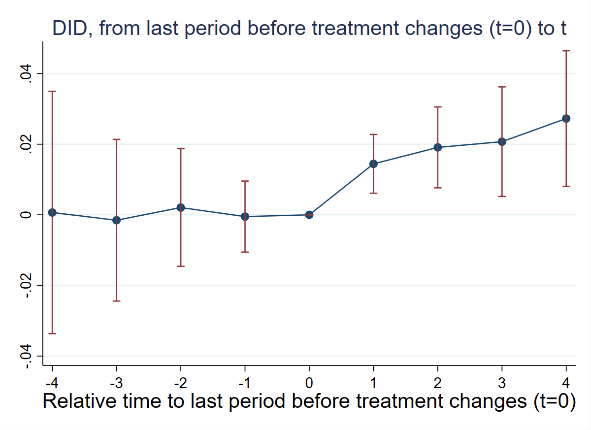
library(haven); library(polars); library(DIDmultiplegtDYN)
load(url("https://raw.githubusercontent.com/Credible-Answers/did_book/main/cc_xd_didtextbook_2025_9_30/Data%20sets/Gentzkow%20et%20al%202011/gentzkowetal_didtextbook.RData"))
gq4 <- did_multiplegt_dyn(
  df = df, outcome = "prestout", group = "cnty90",
  time = "year", treatment = "numdailies",
  effects = 4, placebo = 4, effects_equal = TRUE, cluster = "cnty90")
ggsave("figures/ch08_fig81_nonnormalized_es_R.png",
       plot = gq4$plot, width = 8, height = 5, dpi = 150)
Estimate SE LB CI UB CI N Switchers
Effect_1 0.01442 0.00425 0.00610 0.02275 5,674 1,119
Effect_2 0.01909 0.00584 0.00764 0.03054 4,648 1,054
Effect_3 0.02071 0.00792 0.00520 0.03623 3,750 984
Effect_4 0.02727 0.00979 0.00807 0.04646 2,980 917
Test of joint nullity of the effects : p-value = 0.0068
Test of equality of the effects : p-value = 0.4152
Av_tot_eff = 0.01606 (SE = 0.00478)
Placebo_1 -0.00050 0.00513 4,471 902
Placebo_2 0.00206 0.00850 2,778 746
Placebo_3 -0.00154 0.01168 1,644 604
Placebo_4 0.00066 0.01750 910 441
Test of joint nullity of the placebos : p-value = 0.9922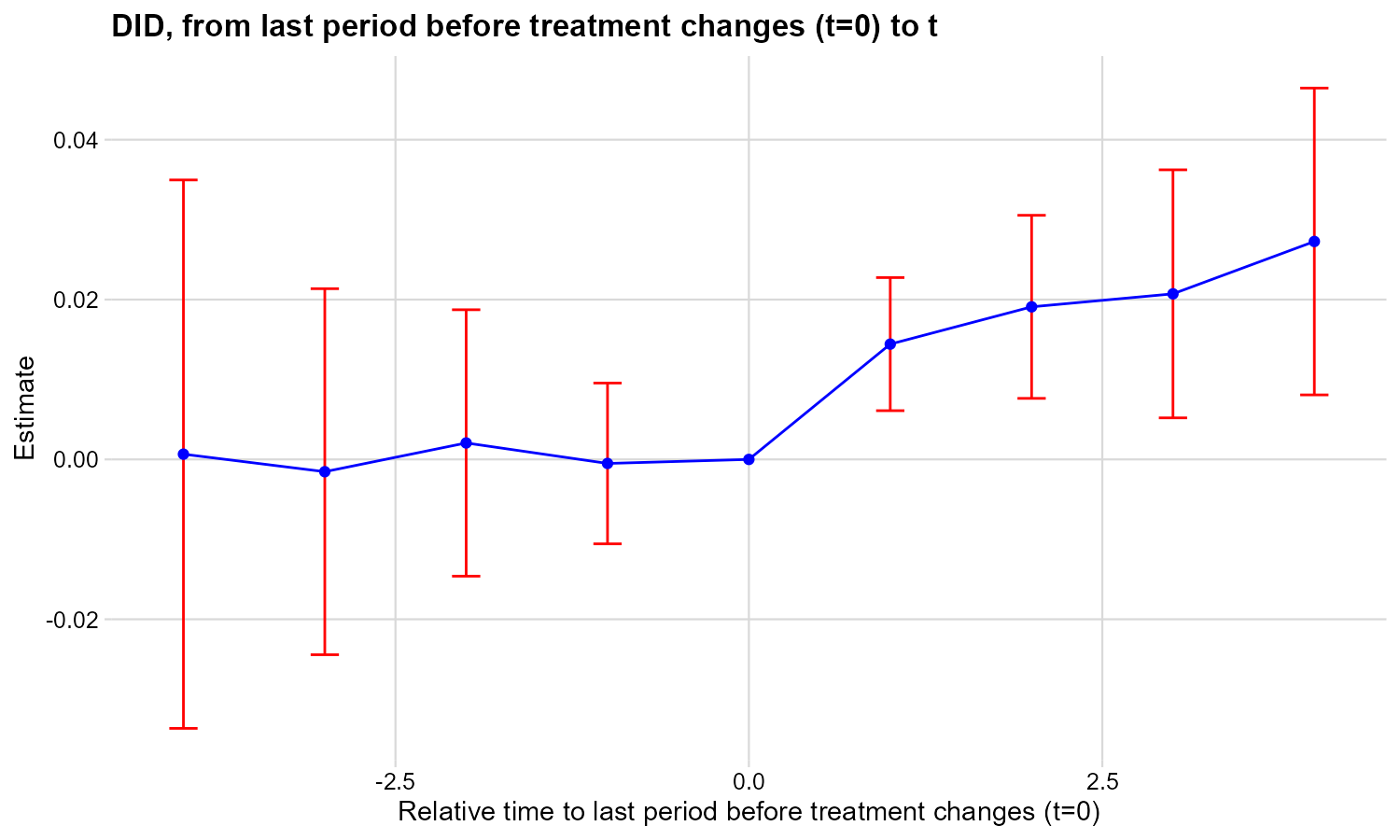
import pandas as pd
import polars as pl
import matplotlib.pyplot as plt
from did_multiplegt_dyn import DidMultiplegtDyn
df = pd.read_parquet("https://raw.githubusercontent.com/Credible-Answers/did_book/main/cc_xd_didtextbook_2025_9_30/Data%20sets/Gentzkow%20et%20al%202011/gentzkowetal_didtextbook.parquet")
df_pl = pl.from_pandas(df)
pd.set_option('display.float_format', lambda x: f'{x:.7f}')
gq4 = DidMultiplegtDyn(df=df_pl, outcome="prestout", group="cnty90",
    time="year", treatment="numdailies", effects=4, placebo=4, effects_equal=True, cluster="cnty90")
gq4.fit(); gq4.summary()
gq4.plot()
plt.savefig("figures/ch08_fig81_nonnormalized_es_Python.png", dpi=150, bbox_inches="tight")
Block Estimate SE LB CI UB CI N Switchers
Effect_1 0.0144244 0.0042477 0.0060992 0.0227497 5674 1119
Effect_2 0.0190899 0.0058429 0.0076381 0.0305418 4648 1054
Effect_3 0.0207147 0.0079164 0.0051989 0.0362305 3750 984
Effect_4 0.0272653 0.0097924 0.0080727 0.0464580 2980 917
Average_Total_Effect 0.0160565 0.0047761 0.0066956 0.0254174 8659 4074
Placebo_1 -0.0005025 0.0051322 -0.0105615 0.0095565 4471 902
Placebo_2 0.0020594 0.0085031 -0.0146063 0.0187251 2778 746
Placebo_3 -0.0015365 0.0116825 -0.0244337 0.0213607 1644 604
Placebo_4 0.0006573 0.0175032 -0.0336483 0.0349628 910 441
Test of joint nullity of the effects : p-value = 0.006814
Test of joint nullity of the placebos: p-value = 0.992198
Test of equality of the effects: p-value = 0.415152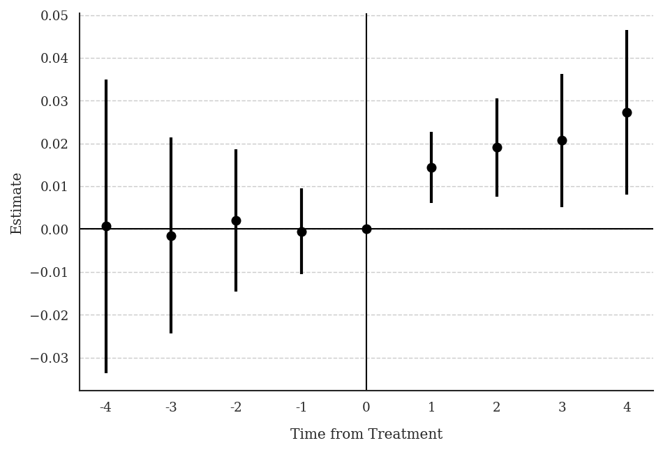
Interpretation: All four non-normalized event-study effects are positive and significant, suggesting newspapers increase turnout. The effects grow with \(\ell\), from 0.0144 at \(\ell = 1\) to 0.0273 at \(\ell = 4\). However, one cannot reject the null that all effects are equal (p-value = 0.4152). All placebo estimates are small and insignificant, with a joint p-value of 0.9922, strongly supporting the parallel-trends assumption. The average cumulative effect per treatment unit is 0.0161 (SE = 0.0048).
CQ#43: Detecting Treatment Paths
Rerun the previous command, estimating one event-study effect and adding
design(0.8,console)at the end, to see the most common treatment paths that together account for 80% of switchers’ \((F_g - 1)\)-to-\(F_g\) paths. Rerun the previous command, estimating two event-study effects. Rerun the previous command, estimating four event-study effects.
* ssc install did_multiplegt_dyn, replace
copy "https://raw.githubusercontent.com/Credible-Answers/did_book/main/cc_xd_didtextbook_2025_9_30/Data%20sets/Gentzkow%20et%20al%202011/gentzkowetal_didtextbook.dta" "gentzkowetal_didtextbook.dta", replace
use "gentzkowetal_didtextbook.dta", clear
did_multiplegt_dyn prestout cnty90 year numdailies, effects(1) design(0.8,console) graph_off
--------------------------------------------------------------------------------
             Estimation of treatment effects: Event-study effects
--------------------------------------------------------------------------------

             |  Estimate         SE      LB CI      UB CI          N  Switchers
-------------+-----------------------------------------------------------------
    Effect_1 |  .0144244   .0042477   .0060992   .0227497       5674       1119
--------------------------------------------------------------------------------


--------------------------------------------------------------------------------
               Average cumulative (total) effect per treatment unit
--------------------------------------------------------------------------------

             |  Estimate         SE      LB CI      UB CI          N     Switch  x Periods
-------------+----------------------------------------------------------------------------
  Av_tot_eff |  .0120186   .0035392   .0050819   .0189552       5674       1119
--------------------------------------------------------------------------------
Average number of time periods over which a treatment's effect is accumulated = 1


--------------------------------------------------------------------------------
          Detection of treatment paths - 1 periods after first switch
--------------------------------------------------------------------------------

             |   #Groups    %Groups        ℓ=0        ℓ=1
-------------+-------------------------------------------
  TreatPath1 |       721      64.03          0          1
  TreatPath2 |       139      12.34          0          2
  TreatPath3 |        54      4.796          1          2
--------------------------------------------------------------------------------
 Treatment paths detected in at least 80.00% of the switching groups 1126 for which 1 effects could be estimated.
 Total % = 81.17 %
 Design interpretation (first row):
 721 groups started with treatment 0 and then experienced treatment 1.
did_multiplegt_dyn prestout cnty90 year numdailies, effects(2) design(0.8,console) graph_off
--------------------------------------------------------------------------------
             Estimation of treatment effects: Event-study effects
--------------------------------------------------------------------------------

             |  Estimate         SE      LB CI      UB CI          N  Switchers
-------------+-----------------------------------------------------------------
    Effect_1 |  .0144244   .0042477   .0060992   .0227497       5674       1119
    Effect_2 |  .0190899   .0058429   .0076381   .0305418       4648       1054
--------------------------------------------------------------------------------
Test of joint nullity of the effects : p-value = .00148173


--------------------------------------------------------------------------------
               Average cumulative (total) effect per treatment unit
--------------------------------------------------------------------------------

             |  Estimate         SE      LB CI      UB CI          N     Switch  x Periods
-------------+----------------------------------------------------------------------------
  Av_tot_eff |   .014327    .003989   .0065087   .0221454       6754       2173
--------------------------------------------------------------------------------
Average number of time periods over which a treatment's effect is accumulated = 1.5211379


--------------------------------------------------------------------------------
          Detection of treatment paths - 2 periods after first switch
--------------------------------------------------------------------------------

             |   #Groups    %Groups        ℓ=0        ℓ=1        ℓ=2
-------------+------------------------------------------------------
  TreatPath1 |       343      32.15          0          1          1
  TreatPath2 |       187      17.53          0          1          0
  TreatPath3 |       131      12.28          0          1          2
  TreatPath4 |        57      5.342          0          2          2
  TreatPath5 |        47      4.405          0          2          1
  TreatPath6 |        33      3.093          1          2          2
  TreatPath7 |        30      2.812          0          1          3
  TreatPath8 |        22      2.062          2          3          2
  TreatPath9 |        20      1.874          2          1          1
--------------------------------------------------------------------------------
 Treatment paths detected in at least 80.00% of the switching groups 1067 for which 2 effects could be estimated.
 Total % = 81.54 %
 Design interpretation (first row):
 343 groups started with treatment 0 and then experienced treatment vector (1, 1).
did_multiplegt_dyn prestout cnty90 year numdailies, effects(4) design(0.8,console) graph_off
--------------------------------------------------------------------------------
             Estimation of treatment effects: Event-study effects
--------------------------------------------------------------------------------

             |  Estimate         SE      LB CI      UB CI          N  Switchers
-------------+-----------------------------------------------------------------
    Effect_1 |  .0144244   .0042477   .0060992   .0227497       5674       1119
    Effect_2 |  .0190899   .0058429   .0076381   .0305418       4648       1054
    Effect_3 |  .0207147   .0079164   .0051989   .0362305       3750        984
    Effect_4 |  .0272653   .0097924   .0080727    .046458       2980        917
--------------------------------------------------------------------------------
Test of joint nullity of the effects : p-value = .00681389


--------------------------------------------------------------------------------
               Average cumulative (total) effect per treatment unit
--------------------------------------------------------------------------------

             |  Estimate         SE      LB CI      UB CI          N     Switch  x Periods
-------------+----------------------------------------------------------------------------
  Av_tot_eff |  .0160565   .0047761   .0066956   .0254174       8659       4074
--------------------------------------------------------------------------------
Average number of time periods over which a treatment's effect is accumulated = 2.4375615


--------------------------------------------------------------------------------
          Detection of treatment paths - 4 periods after first switch
--------------------------------------------------------------------------------

             |   #Groups    %Groups        ℓ=0        ℓ=1        ℓ=2        ℓ=3        ℓ=4
-------------+----------------------------------------------------------------------------
  TreatPath1 |       141      15.11          0          1          1          1          1
  TreatPath2 |       127      13.61          0          1          0          0          0
  TreatPath3 |        43      4.609          0          1          2          2          2
  TreatPath4 |        40      4.287          0          1          1          1          2
  TreatPath5 |        32       3.43          0          1          1          2          2
  TreatPath6 |        19      2.036          0          1          2          1          1
  TreatPath7 |        18      1.929          0          1          1          1          0
  TreatPath8 |        18      1.929          0          2          1          1          1
  TreatPath9 |        16      1.715          0          1          1          0          0
 TreatPath10 |        16      1.715          0          2          2          2          2
 TreatPath11 |        15      1.608          0          1          0          0          1
 TreatPath12 |        15      1.608          0          1          1          2          1
 TreatPath13 |        15      1.608          0          1          2          2          1
 TreatPath14 |        12      1.286          0          1          0          1          1
 TreatPath15 |        12      1.286          0          2          1          2          2
 TreatPath16 |        11      1.179          0          1          2          1          2
 TreatPath17 |        10      1.072          1          2          2          2          2
 TreatPath18 |         8      .8574          0          1          2          2          3
 TreatPath19 |         8      .8574          0          2          2          1          1
 TreatPath20 |         8      .8574          1          0          0          0          0
 TreatPath21 |         7      .7503          0          1          1          0          1
 TreatPath22 |         7      .7503          0          1          1          3          3
 TreatPath23 |         7      .7503          0          1          2          3          2
 TreatPath24 |         7      .7503          0          1          2          3          3
 TreatPath25 |         7      .7503          0          1          3          2          2
 TreatPath26 |         6      .6431          0          1          0          1          2
 TreatPath27 |         6      .6431          0          1          1          2          3
 TreatPath28 |         6      .6431          0          2          0          0          0
 TreatPath29 |         6      .6431          0          2          2          3          2
 TreatPath30 |         6      .6431          1          2          2          2          1
 TreatPath31 |         6      .6431          2          1          1          1          1
 TreatPath32 |         5      .5359          0          1          3          3          3
 TreatPath33 |         5      .5359          0          2          1          1          2
 TreatPath34 |         5      .5359          0          2          2          1          2
 TreatPath35 |         5      .5359          0          2          2          2          3
 TreatPath36 |         5      .5359          0          2          3          2          2
 TreatPath37 |         5      .5359          2          3          2          2          2
 TreatPath38 |         4      .4287          0          1          1          1          3
 TreatPath39 |         4      .4287          0          1          3          2          3
 TreatPath40 |         4      .4287          0          2          2          2          1
 TreatPath41 |         4      .4287          0          2          2          3          3
 TreatPath42 |         4      .4287          0          3          2          3          2
 TreatPath43 |         4      .4287          1          2          2          3          3
 TreatPath44 |         3      .3215          0          1          0          0          2
 TreatPath45 |         3      .3215          0          1          0          1          0
 TreatPath46 |         3      .3215          0          1          1          0          2
 TreatPath47 |         3      .3215          0          1          1          2          4
 TreatPath48 |         3      .3215          0          1          1          3          2
 TreatPath49 |         3      .3215          0          1          3          3          2
 TreatPath50 |         3      .3215          0          2          1          2          1
 TreatPath51 |         3      .3215          0          2          3          4          3
 TreatPath52 |         3      .3215          1          0          0          0          1
 TreatPath53 |         3      .3215          1          2          1          2          2
 TreatPath54 |         3      .3215          1          2          2          1          1
 TreatPath55 |         3      .3215          1          2          2          2          3
 TreatPath56 |         3      .3215          2          1          1          2          2
--------------------------------------------------------------------------------
 Treatment paths detected in at least 80.00% of the switching groups 933 for which 4 effects could be estimated.
 Total % = 80.17 %
 Design interpretation (first row):
141 groups started with treatment 0 and then experienced treatment vector (1, 1, 1, 1).library(haven); library(polars); library(DIDmultiplegtDYN)
load(url("https://raw.githubusercontent.com/Credible-Answers/did_book/main/cc_xd_didtextbook_2025_9_30/Data%20sets/Gentzkow%20et%20al%202011/gentzkowetal_didtextbook.RData")); df <- as.data.frame(df)
gq5_l1 <- did_multiplegt_dyn(df=df, outcome="prestout", group="cnty90",
time="year", treatment="numdailies", effects=1,
design=c(0.8,"console"), graph_off=TRUE)
print(gq5_l1)----------------------------------------------------------------------
Estimation of treatment effects: Event-study effects
----------------------------------------------------------------------
Estimate SE LB CI UB CI N Switchers
0.01442 0.00425 0.00610 0.02275 5,674 1,119
----------------------------------------------------------------------
Average cumulative (total) effect per treatment unit
----------------------------------------------------------------------
Estimate SE LB CI UB CI N Switchers
0.01202 0.00354 0.00508 0.01896 5,674 1,119
Average number of time periods over which a treatment effect is accumulated: 1.0000
----------------------------------------------------------------------
Detection of treatment paths - 1 periods after first switch
----------------------------------------------------------------------
N Share ℓ=0 ℓ=1
TreatPath1 721 64.03 0 1
TreatPath2 139 12.34 0 2
TreatPath3 54 4.80 1 2
Treatment paths detected in at least 80.00% of the 1126 switching groups for which 1 effects could be estimated (Total % = 81.17%)
Design interpretation (first row):
721 groups started with treatment 0 and experienced treatment path (1)gq5_l2 <- did_multiplegt_dyn(df=df, outcome="prestout", group="cnty90",
time="year", treatment="numdailies", effects=2,
design=c(0.8,"console"), graph_off=TRUE)
print(gq5_l2)----------------------------------------------------------------------
Estimation of treatment effects: Event-study effects
----------------------------------------------------------------------
Estimate SE LB CI UB CI N Switchers
Effect_1 0.01442 0.00425 0.00610 0.02275 5,674 1,119
Effect_2 0.01909 0.00584 0.00764 0.03054 4,648 1,054
Test of joint nullity of the effects : p-value = 0.0015
----------------------------------------------------------------------
Average cumulative (total) effect per treatment unit
----------------------------------------------------------------------
Estimate SE LB CI UB CI N Switchers
0.01433 0.00399 0.00651 0.02215 6,754 2,173
Average number of time periods over which a treatment effect is accumulated: 1.5211
----------------------------------------------------------------------
Detection of treatment paths - 2 periods after first switch
----------------------------------------------------------------------
N Share ℓ=0 ℓ=1 ℓ=2
TreatPath1 343 32.15 0 1 1
TreatPath2 187 17.53 0 1 0
TreatPath3 131 12.28 0 1 2
TreatPath4 57 5.34 0 2 2
TreatPath5 47 4.40 0 2 1
TreatPath6 33 3.09 1 2 2
TreatPath7 30 2.81 0 1 3
TreatPath8 22 2.06 2 3 2
TreatPath9 20 1.87 2 1 1
Treatment paths detected in at least 80.00% of the 1067 switching groups for which 2 effects could be estimated (Total % = 81.54%)
Design interpretation (first row):
343 groups started with treatment 0 and experienced treatment path (1,1)gq5_l4 <- did_multiplegt_dyn(df=df, outcome="prestout", group="cnty90",
time="year", treatment="numdailies", effects=4,
design=c(0.8,"console"), graph_off=TRUE)
print(gq5_l4)----------------------------------------------------------------------
Estimation of treatment effects: Event-study effects
----------------------------------------------------------------------
Estimate SE LB CI UB CI N Switchers
Effect_1 0.01442 0.00425 0.00610 0.02275 5,674 1,119
Effect_2 0.01909 0.00584 0.00764 0.03054 4,648 1,054
Effect_3 0.02071 0.00792 0.00520 0.03623 3,750 984
Effect_4 0.02727 0.00979 0.00807 0.04646 2,980 917
Test of joint nullity of the effects : p-value = 0.0068
----------------------------------------------------------------------
Average cumulative (total) effect per treatment unit
----------------------------------------------------------------------
Estimate SE LB CI UB CI N Switchers
0.01606 0.00478 0.00670 0.02542 8,659 4,074
Average number of time periods over which a treatment effect is accumulated: 2.4376
----------------------------------------------------------------------
Detection of treatment paths - 4 periods after first switch
----------------------------------------------------------------------
N Share ℓ=0 ℓ=1 ℓ=2 ℓ=3 ℓ=4
TreatPath1 141 15.11 0 1 1 1 1
TreatPath2 127 13.61 0 1 0 0 0
TreatPath3 43 4.61 0 1 2 2 2
TreatPath4 40 4.29 0 1 1 1 2
TreatPath5 32 3.43 0 1 1 2 2
TreatPath6 19 2.04 0 1 2 1 1
TreatPath7 18 1.93 0 1 1 1 0
TreatPath8 18 1.93 0 2 1 1 1
TreatPath9 16 1.71 0 1 1 0 0
TreatPath10 16 1.71 0 2 2 2 2
TreatPath11 15 1.61 0 1 0 0 1
TreatPath12 15 1.61 0 1 1 2 1
TreatPath13 15 1.61 0 1 2 2 1
TreatPath14 12 1.29 0 1 0 1 1
TreatPath15 12 1.29 0 2 1 2 2
TreatPath16 11 1.18 0 1 2 1 2
TreatPath17 10 1.07 1 2 2 2 2
TreatPath18 8 0.86 0 1 2 2 3
TreatPath19 8 0.86 0 2 2 1 1
TreatPath20 8 0.86 1 0 0 0 0
TreatPath21 7 0.75 0 1 1 0 1
TreatPath22 7 0.75 0 1 1 3 3
TreatPath23 7 0.75 0 1 2 3 2
TreatPath24 7 0.75 0 1 2 3 3
TreatPath25 7 0.75 0 1 3 2 2
TreatPath26 6 0.64 0 1 0 1 2
TreatPath27 6 0.64 0 1 1 2 3
TreatPath28 6 0.64 0 2 0 0 0
TreatPath29 6 0.64 0 2 2 3 2
TreatPath30 6 0.64 1 2 2 2 1
TreatPath31 6 0.64 2 1 1 1 1
TreatPath32 5 0.54 0 1 3 3 3
TreatPath33 5 0.54 0 2 1 1 2
TreatPath34 5 0.54 0 2 2 1 2
TreatPath35 5 0.54 0 2 2 2 3
TreatPath36 5 0.54 0 2 3 2 2
TreatPath37 5 0.54 2 3 2 2 2
TreatPath38 4 0.43 0 1 1 1 3
TreatPath39 4 0.43 0 1 3 2 3
TreatPath40 4 0.43 0 2 2 2 1
TreatPath41 4 0.43 0 2 2 3 3
TreatPath42 4 0.43 0 3 2 3 2
TreatPath43 4 0.43 1 2 2 3 3
TreatPath44 3 0.32 0 1 0 0 2
TreatPath45 3 0.32 0 1 0 1 0
TreatPath46 3 0.32 0 1 1 0 2
TreatPath47 3 0.32 0 1 1 2 4
TreatPath48 3 0.32 0 1 1 3 2
TreatPath49 3 0.32 0 1 3 3 2
TreatPath50 3 0.32 0 2 1 2 1
TreatPath51 3 0.32 0 2 3 4 3
TreatPath52 3 0.32 1 0 0 0 1
TreatPath53 3 0.32 1 2 1 2 2
TreatPath54 3 0.32 1 2 2 1 1
TreatPath55 3 0.32 1 2 2 2 3
TreatPath56 3 0.32 2 1 1 2 2
Treatment paths detected in at least 80.00% of the 933 switching groups for which 4 effects could be estimated (Total % = 80.17%)
Design interpretation (first row):
141 groups started with treatment 0 and experienced treatment path (1,1,1,1)import pandas as pd
import polars as pl
from did_multiplegt_dyn import DidMultiplegtDyn
df = pd.read_parquet("https://raw.githubusercontent.com/Credible-Answers/did_book/main/cc_xd_didtextbook_2025_9_30/Data%20sets/Gentzkow%20et%20al%202011/gentzkowetal_didtextbook.parquet")
df_pl = pl.from_pandas(df)
pd.set_option('display.float_format', lambda x: f'{x:.7f}')
for ell in [1, 2, 4]:
model = DidMultiplegtDyn(df=df_pl, outcome="prestout", group="cnty90",
time="year", treatment="numdailies", effects=ell, cluster="cnty90",
design=[0.8, "console"])
model.fit(); model.summary()================================================================================
Detection of treatment paths - 1 periods after first switch
================================================================================
#Groups %Groups l=0 l=1
TreatPath1 721 64.0319716 0.0000000 1.0000000
TreatPath2 139 12.3445826 0.0000000 2.0000000
TreatPath3 54 4.7957371 2.0000000 3.0000000
TreatPath4 54 4.7957371 1.0000000 2.0000000
================================================================================
Treatment paths detected in switching groups: 1126
Total % shown: 85.97%
Design interpretation (first row):
721 groups started with treatment 0.0 and then experienced treatment [np.float64(1.0)]
================================================================================
Estimation of treatment effects: Event-study effects
================================================================================
Block Estimate SE LB CI UB CI N Switchers N.w Switchers.w
Effect_1 0.0144244 0.0042477 0.0060992 0.0227497 5674.0000000 1119.0000000 5674.0000000 1119.0000000
Average_Total_Effect 0.0120186 0.0035392 0.0050819 0.0189552 5674.0000000 1119.0000000 5674.0000000 1119.0000000
Placebo_1 -0.0005025 0.0051322 -0.0105615 0.0095565 4471.0000000 902.0000000 4471.0000000 902.0000000
================================================================================
The development of this package was funded by the European Union.
ERC REALLYCREDIBLE - GA N. 101043899
================================================================================
Detection of treatment paths - 2 periods after first switch
================================================================================
#Groups %Groups l=0 l=1 l=2
TreatPath1 343 32.1462043 0.0000000 1.0000000 1.0000000
TreatPath2 187 17.5257732 0.0000000 1.0000000 0.0000000
TreatPath3 131 12.2774133 0.0000000 1.0000000 2.0000000
TreatPath4 57 5.3420806 0.0000000 2.0000000 2.0000000
TreatPath5 47 4.4048735 0.0000000 2.0000000 1.0000000
TreatPath6 33 3.0927835 1.0000000 2.0000000 2.0000000
TreatPath7 30 2.8116214 0.0000000 1.0000000 3.0000000
TreatPath8 22 2.0618557 2.0000000 3.0000000 2.0000000
TreatPath9 20 1.8744142 2.0000000 1.0000000 1.0000000
TreatPath10 18 1.6869728 2.0000000 3.0000000 3.0000000
================================================================================
Treatment paths detected in switching groups: 1067
Total % shown: 83.22%
Design interpretation (first row):
343 groups started with treatment 0.0 and then experienced treatment [np.float64(1.0), np.float64(1.0)]
================================================================================
Estimation of treatment effects: Event-study effects
================================================================================
Block Estimate SE LB CI UB CI N Switchers N.w Switchers.w
Effect_1 0.0144244 0.0042477 0.0060992 0.0227497 5674.0000000 1119.0000000 5674.0000000 1119.0000000
Effect_2 0.0190899 0.0058429 0.0076381 0.0305418 4648.0000000 1054.0000000 4648.0000000 1054.0000000
Average_Total_Effect 0.0143270 0.0039890 0.0065087 0.0221454 6754.0000000 2173.0000000 6754.0000000 2173.0000000
Placebo_1 -0.0005025 0.0051322 -0.0105615 0.0095565 4471.0000000 902.0000000 4471.0000000 902.0000000
================================================================================
Test of joint nullity of the effects: p-value = 0.001482
The development of this package was funded by the European Union.
ERC REALLYCREDIBLE - GA N. 101043899
================================================================================
Detection of treatment paths - 4 periods after first switch
================================================================================
#Groups %Groups l=0 l=1 l=2 l=3 l=4
TreatPath1 141 15.1125402 0.0000000 1.0000000 1.0000000 1.0000000 1.0000000
TreatPath2 127 13.6120043 0.0000000 1.0000000 0.0000000 0.0000000 0.0000000
TreatPath3 43 4.6087889 0.0000000 1.0000000 2.0000000 2.0000000 2.0000000
TreatPath4 40 4.2872454 0.0000000 1.0000000 1.0000000 1.0000000 2.0000000
TreatPath5 32 3.4297964 0.0000000 1.0000000 1.0000000 2.0000000 2.0000000
TreatPath6 19 2.0364416 0.0000000 1.0000000 2.0000000 1.0000000 1.0000000
TreatPath7 18 1.9292605 0.0000000 2.0000000 1.0000000 1.0000000 1.0000000
TreatPath8 18 1.9292605 0.0000000 1.0000000 1.0000000 1.0000000 0.0000000
TreatPath9 16 1.7148982 0.0000000 1.0000000 1.0000000 0.0000000 0.0000000
TreatPath10 16 1.7148982 0.0000000 2.0000000 2.0000000 2.0000000 2.0000000
TreatPath11 15 1.6077170 0.0000000 1.0000000 0.0000000 0.0000000 1.0000000
TreatPath12 15 1.6077170 0.0000000 1.0000000 1.0000000 2.0000000 1.0000000
TreatPath13 15 1.6077170 0.0000000 1.0000000 2.0000000 2.0000000 1.0000000
TreatPath14 12 1.2861736 0.0000000 1.0000000 0.0000000 1.0000000 1.0000000
TreatPath15 12 1.2861736 0.0000000 2.0000000 1.0000000 2.0000000 2.0000000
TreatPath16 11 1.1789925 0.0000000 1.0000000 2.0000000 1.0000000 2.0000000
TreatPath17 10 1.0718114 1.0000000 2.0000000 2.0000000 2.0000000 2.0000000
TreatPath18 8 0.8574491 0.0000000 2.0000000 2.0000000 1.0000000 1.0000000
TreatPath19 8 0.8574491 1.0000000 0.0000000 0.0000000 0.0000000 0.0000000
TreatPath20 8 0.8574491 0.0000000 1.0000000 2.0000000 2.0000000 3.0000000
TreatPath21 7 0.7502680 0.0000000 1.0000000 2.0000000 3.0000000 2.0000000
TreatPath22 7 0.7502680 0.0000000 1.0000000 1.0000000 0.0000000 1.0000000
TreatPath23 7 0.7502680 0.0000000 1.0000000 3.0000000 2.0000000 2.0000000
TreatPath24 7 0.7502680 0.0000000 1.0000000 1.0000000 3.0000000 3.0000000
TreatPath25 7 0.7502680 0.0000000 1.0000000 2.0000000 3.0000000 3.0000000
TreatPath26 6 0.6430868 1.0000000 2.0000000 2.0000000 2.0000000 1.0000000
TreatPath27 6 0.6430868 0.0000000 2.0000000 2.0000000 3.0000000 2.0000000
TreatPath28 6 0.6430868 0.0000000 2.0000000 0.0000000 0.0000000 0.0000000
TreatPath29 6 0.6430868 0.0000000 1.0000000 0.0000000 1.0000000 2.0000000
TreatPath30 6 0.6430868 0.0000000 1.0000000 1.0000000 2.0000000 3.0000000
TreatPath31 6 0.6430868 2.0000000 1.0000000 1.0000000 1.0000000 1.0000000
TreatPath32 5 0.5359057 0.0000000 2.0000000 2.0000000 1.0000000 2.0000000
TreatPath33 5 0.5359057 0.0000000 2.0000000 3.0000000 2.0000000 2.0000000
TreatPath34 5 0.5359057 0.0000000 1.0000000 3.0000000 3.0000000 3.0000000
TreatPath35 5 0.5359057 0.0000000 2.0000000 2.0000000 2.0000000 3.0000000
TreatPath36 5 0.5359057 2.0000000 3.0000000 2.0000000 2.0000000 2.0000000
TreatPath37 5 0.5359057 0.0000000 2.0000000 1.0000000 1.0000000 2.0000000
TreatPath38 4 0.4287245 0.0000000 3.0000000 2.0000000 3.0000000 2.0000000
TreatPath39 4 0.4287245 0.0000000 2.0000000 2.0000000 3.0000000 3.0000000
TreatPath40 4 0.4287245 1.0000000 2.0000000 2.0000000 3.0000000 3.0000000
TreatPath41 4 0.4287245 0.0000000 1.0000000 3.0000000 2.0000000 3.0000000
TreatPath42 4 0.4287245 0.0000000 1.0000000 1.0000000 1.0000000 3.0000000
TreatPath43 4 0.4287245 0.0000000 2.0000000 2.0000000 2.0000000 1.0000000
TreatPath44 3 0.3215434 2.0000000 1.0000000 1.0000000 2.0000000 2.0000000
TreatPath45 3 0.3215434 1.0000000 2.0000000 2.0000000 1.0000000 1.0000000
TreatPath46 3 0.3215434 2.0000000 3.0000000 2.0000000 2.0000000 4.0000000
TreatPath47 3 0.3215434 2.0000000 3.0000000 3.0000000 3.0000000 3.0000000
TreatPath48 3 0.3215434 0.0000000 1.0000000 1.0000000 0.0000000 2.0000000
TreatPath49 3 0.3215434 2.0000000 3.0000000 2.0000000 3.0000000 2.0000000
TreatPath50 3 0.3215434 0.0000000 1.0000000 1.0000000 3.0000000 2.0000000
TreatPath51 3 0.3215434 0.0000000 1.0000000 0.0000000 0.0000000 2.0000000
TreatPath52 3 0.3215434 2.0000000 3.0000000 3.0000000 4.0000000 3.0000000
TreatPath53 3 0.3215434 0.0000000 1.0000000 0.0000000 1.0000000 0.0000000
TreatPath54 3 0.3215434 1.0000000 2.0000000 1.0000000 2.0000000 2.0000000
TreatPath55 3 0.3215434 2.0000000 1.0000000 2.0000000 2.0000000 2.0000000
TreatPath56 3 0.3215434 0.0000000 1.0000000 1.0000000 2.0000000 4.0000000
TreatPath57 3 0.3215434 2.0000000 3.0000000 3.0000000 3.0000000 2.0000000
================================================================================
Treatment paths detected in switching groups: 933
Total % shown: 80.49%
Design interpretation (first row):
141 groups started with treatment 0.0 and then experienced treatment [np.float64(1.0), np.float64(1.0), np.float64(1.0), np.float64(1.0)]
================================================================================
Estimation of treatment effects: Event-study effects
================================================================================
Block Estimate SE LB CI UB CI N Switchers N.w Switchers.w
Effect_1 0.0144244 0.0042477 0.0060992 0.0227497 5674.0000000 1119.0000000 5674.0000000 1119.0000000
Effect_2 0.0190899 0.0058429 0.0076381 0.0305418 4648.0000000 1054.0000000 4648.0000000 1054.0000000
Effect_3 0.0207147 0.0079164 0.0051989 0.0362305 3750.0000000 984.0000000 3750.0000000 984.0000000
Effect_4 0.0272653 0.0097924 0.0080727 0.0464580 2980.0000000 917.0000000 2980.0000000 917.0000000
Average_Total_Effect 0.0160565 0.0047761 0.0066956 0.0254174 8659.0000000 4074.0000000 8659.0000000 4074.0000000
Placebo_1 -0.0005025 0.0051322 -0.0105615 0.0095565 4471.0000000 902.0000000 4471.0000000 902.0000000
================================================================================
Test of joint nullity of the effects: p-value = 0.006814
The development of this package was funded by the European Union.
ERC REALLYCREDIBLE - GA N. 101043899CQ#44: Interpreting the Treatment Paths
Interpret the results of the previous estimations: what are the three most common “actual-versus-status-quo” comparisons averaged in \(AVSQ_1\)? In \(AVSQ_2\)? In \(AVSQ_4\)?
Each row of the design output compares a group’s actual treatment path from \(F_g\) to \(F_g - 1 + \ell\) with its status-quo path, in which the treatment would have stayed at its period-\((F_g - 1)\) value.
| Most common | Second | Third | Top 3 share | |
|---|---|---|---|---|
| \(AVSQ_1\) | 1 vs. 0 newspapers (64.0%) | 2 vs. 0 (12.3%) | 2 vs. 1 (4.8%) | 81.2% |
| \(AVSQ_2\) | (1,1) vs. (0,0) (32.1%) | (1,0) vs. (0,0) (17.5%) | (1,2) vs. (0,0) (12.3%) | 62.0% |
| \(AVSQ_4\) | (1,1,1,1) vs. (0,0,0,0) (15.1%) | (1,0,0,0) vs. (0,0,0,0) (13.6%) | (1,2,2,2) vs. (0,0,0,0) (4.6%) | 33.3% |
Interpretation: \(AVSQ_1\) mostly compares counties going from zero to one newspaper with counties that would have kept zero. As \(\ell\) increases, the paths being compared become much more heterogeneous: by \(\ell = 4\), the three most common paths account for only a third of switchers. Some counties gain a newspaper and keep it, while others gain one and lose it right after (the second most common path at \(\ell = 2\) and \(\ell = 4\)). Hence, \(AVSQ_4\) averages effects of very different treatment paths, which complicates its interpretation.
CQ#45: Path-Specific Event-Study Effects (by_path)
Estimate the first two event-study effects separately for the three most common \((D_{g,F_g-1}, D_{g,F_g}, D_{g,F_g+1})\) paths shared by more than 100 counties, using
by_path(3).
copy "https://raw.githubusercontent.com/Credible-Answers/did_book/main/cc_xd_didtextbook_2025_9_30/Data%20sets/Gentzkow%20et%20al%202011/gentzkowetal_didtextbook.dta" "gentzkowetal_didtextbook.dta", replace
use "gentzkowetal_didtextbook.dta", clear
did_multiplegt_dyn prestout cnty90 year numdailies, effects(2) by_path(3)
--- Path (0, 1, 1) ---
| Estimate SE LB CI UB CI N Switchers
Effect_1 | .0131318 .0071358 -.0008542 .0271178 4529 343
Effect_2 | .009357 .0090553 -.008391 .027105 3713 343
Test of joint nullity of the effects : p-value = .1750087
--- Path (0, 1, 0) ---
| Estimate SE LB CI UB CI N Switchers
Effect_1 | .0144984 .0103889 -.0058635 .0348603 4373 187
Effect_2 | .0082605 .0115639 -.0144043 .0309254 3557 187
Test of joint nullity of the effects : p-value = .32227545
--- Path (0, 1, 2) ---
| Estimate SE LB CI UB CI N Switchers
Effect_1 | .0212045 .0103034 .0010102 .0413988 4317 131
Effect_2 | .0314473 .0132732 .0054324 .0574622 3501 131
Test of joint nullity of the effects : p-value = .05711112library(haven); library(DIDmultiplegtDYN)
load(url("https://raw.githubusercontent.com/Credible-Answers/did_book/main/cc_xd_didtextbook_2025_9_30/Data%20sets/Gentzkow%20et%20al%202011/gentzkowetal_didtextbook.RData"))
did_multiplegt_dyn(df = as.data.frame(df), outcome = "prestout", group = "cnty90", time = "year", treatment = "numdailies", effects = 2, by_path = 3)--- Path (0, 1, 1) ---
Estimate SE LB CI UB CI N Switchers
Effect_1 0.01313 0.00714 -0.00085 0.02712 4,529 343
Effect_2 0.00936 0.00906 -0.00839 0.02711 3,713 343
Test of joint nullity of the effects : p-value = 0.1750
--- Path (0, 1, 0) ---
Estimate SE LB CI UB CI N Switchers
Effect_1 0.01450 0.01039 -0.00586 0.03486 4,373 187
Effect_2 0.00826 0.01156 -0.01440 0.03093 3,557 187
Test of joint nullity of the effects : p-value = 0.3223
--- Path (0, 1, 2) ---
Estimate SE LB CI UB CI N Switchers
Effect_1 0.02120 0.01030 0.00101 0.04140 4,317 131
Effect_2 0.03145 0.01327 0.00543 0.05746 3,501 131
Test of joint nullity of the effects : p-value = 0.0571import pandas as pd
import polars as pl
from did_multiplegt_dyn import DidMultiplegtDyn
df = pd.read_parquet("https://raw.githubusercontent.com/Credible-Answers/did_book/main/cc_xd_didtextbook_2025_9_30/Data%20sets/Gentzkow%20et%20al%202011/gentzkowetal_didtextbook.parquet")
df_pl = pl.from_pandas(df)
bp = DidMultiplegtDyn(df=df_pl, outcome="prestout", group="cnty90", time="year", treatment="numdailies", effects=2, by_path=3, cluster="cnty90")
bp.fit(); bp.summary() Path (0, 1, 1)
343 switchers
================================================================================
Block Estimate SE LB CI UB CI N Switchers N.w Switchers.w
Effect_1 0.013149 0.007141 -0.000847 0.027146 4477.0 343.0 4477.0 343.0
Effect_2 0.009833 0.009065 -0.007934 0.027601 3673.0 343.0 3673.0 343.0
Average_Total_Effect 0.011491 0.007451 -0.003113 0.026095 4841.0 686.0 4841.0 686.0
Placebo_1 0.002974 0.007324 -0.011381 0.017328 3624.0 315.0 3624.0 315.0
================================================================================
Test of joint nullity of the effects: p-value = 0.178040
Path (0, 1, 0)
187 switchers
================================================================================
Block Estimate SE LB CI UB CI N Switchers N.w Switchers.w
Effect_1 0.014548 0.010391 -0.005817 0.034913 4321.0 187.0 4321.0 187.0
Effect_2 0.008902 0.011569 -0.013773 0.031578 3517.0 187.0 3517.0 187.0
Average_Total_Effect 0.023450 0.020660 -0.017043 0.063943 4529.0 374.0 4529.0 374.0
Placebo_1 -0.010694 0.010761 -0.031784 0.010396 3469.0 160.0 3469.0 160.0
================================================================================
Test of joint nullity of the effects: p-value = 0.334025
Path (0, 1, 2)
131 switchers
================================================================================
Block Estimate SE LB CI UB CI N Switchers N.w Switchers.w
Effect_1 0.021508 0.010305 0.001310 0.041707 4265.0 131.0 4265.0 131.0
Effect_2 0.032215 0.013281 0.006184 0.058245 3461.0 131.0 3461.0 131.0
Average_Total_Effect 0.017908 0.007425 0.003355 0.032460 4417.0 262.0 4417.0 262.0
Placebo_1 0.009111 0.010579 -0.011623 0.029845 3430.0 121.0 3430.0 121.0
================================================================================
Test of joint nullity of the effects: p-value = 0.050280Interpretation: Event-study effects are insignificant for the \((D_{g,F_g-1}, D_{g,F_g}, D_{g,F_g+1}) = (0, 1, 1)\) and \((0, 1, 0)\) paths, and significant for the \((0, 1, 2)\) path. This might suggest that sustained exposure to an increasing number of newspapers is necessary to generate an effect, though event-study effects are noisy and may not significantly differ across paths.
CQ#46: Normalized Event-Study Effects (Figure 8.2)
Compute, for \(\ell \in \{1, \ldots, 4\}\), normalized event-study estimates \(\widehat{AVSQ}^n_\ell\), as well as the weights \(w_{\ell,k}\) that normalized effect \(\ell\) puts on the effect of the \(k\)th treatment lag for \(k \in \{0, \ldots, \ell - 1\}\). Compute also normalized pre-trend estimates \(\widehat{AVSQ}^n_{-\ell}\) for \(\ell \in \{1, \ldots, 4\}\).
* ssc install did_multiplegt_dyn, replace
copy "https://raw.githubusercontent.com/Credible-Answers/did_book/main/cc_xd_didtextbook_2025_9_30/Data%20sets/Gentzkow%20et%20al%202011/gentzkowetal_didtextbook.dta" "gentzkowetal_didtextbook.dta", replace
use "gentzkowetal_didtextbook.dta", clear
did_multiplegt_dyn prestout cnty90 year numdailies, effects(4) placebo(4) normalized effects_equal(all) normalized_weights cluster(cnty90)
graph export "figures\ch08_fig82_normalized_es.png", replace width(1200)
----------------------------------------------------------------------
Estimation of treatment effects: Event-study effects
----------------------------------------------------------------------
Estimate SE LB CI UB CI N Switchers
Effect_1 0.0120186 0.0035392 0.0050819 0.0189552 5,674 1,119
Effect_2 0.0082126 0.0025136 0.0032859 0.0131392 4,648 1,054
Effect_3 0.0057192 0.0021857 0.0014354 0.0100030 3,750 984
Effect_4 0.0053873 0.0019348 0.0015951 0.0091795 2,980 917
Test of joint nullity of the effects : p-value = 0.0068
Test of equality of the effects : p-value = 0.1653
Average cumulative (total) effect per treatment unit:
0.0160565 (SE = 0.0047761)
----------------------------------------------------------------------
Testing the parallel trends and no anticipation assumptions
----------------------------------------------------------------------
Estimate SE LB CI UB CI N Switchers
Placebo_1 -0.0004158 0.0042470 -0.0087399 0.0079082 4,471 902
Placebo_2 0.0008699 0.0035919 -0.0061701 0.0079099 2,778 746
Placebo_3 -0.0004201 0.0031943 -0.0066808 0.0058406 1,644 604
Placebo_4 0.0001394 0.0037128 -0.0071375 0.0074164 910 441
Test of joint nullity of the placebos : p-value = 0.9922
----------------------------------------------------------------------
Weights on treatment lags
----------------------------------------------------------------------
| ℓ=1 ℓ=2 ℓ=3 ℓ=4
k=0 | 1.0000 0.4849 0.3549 0.2777
k=1 | . 0.5151 0.3131 0.2568
k=2 | . . 0.3319 0.2271
k=3 | . . . 0.2383
Total | 1.0000 1.0000 1.0000 1.0000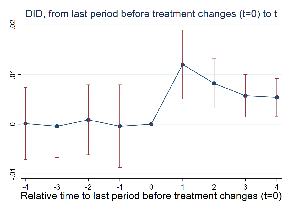
library(haven); library(polars); library(DIDmultiplegtDYN)
load(url("https://raw.githubusercontent.com/Credible-Answers/did_book/main/cc_xd_didtextbook_2025_9_30/Data%20sets/Gentzkow%20et%20al%202011/gentzkowetal_didtextbook.RData")); df <- as.data.frame(df)
gq6 <- did_multiplegt_dyn(
    df = df, outcome = "prestout", group = "cnty90",
    time = "year", treatment = "numdailies",
    effects = 4, placebo = 4,
    normalized = TRUE, normalized_weights = TRUE, effects_equal = TRUE, cluster = "cnty90")
ggsave("figures/ch08_fig82_normalized_es_R.png",
       plot = gq6$plot, width = 8, height = 5, dpi = 150)
Estimate SE LB CI UB CI N Switchers
Effect_1 0.0120186 0.0035392 0.0050818 0.0189554 5,674 1,119
Effect_2 0.0082126 0.0025136 0.0032860 0.0131392 4,648 1,054
Effect_3 0.0057192 0.0021857 0.0014353 0.0100031 3,750 984
Effect_4 0.0053873 0.0019348 0.0015951 0.0091795 2,980 917
Joint nullity of effects : p = 0.0068
Equality of effects : p = 0.1653
Av_tot_eff = 0.0160565 (SE = 0.0047761)
Placebo_1 -0.0004159 0.0042471 4,418 902
Placebo_2 0.0008718 0.0035930 2,764 746
Placebo_3 -0.0004199 0.0031938 1,636 604
Placebo_4 0.0001368 0.0037130 907 441
Joint nullity of placebos : p = 0.9922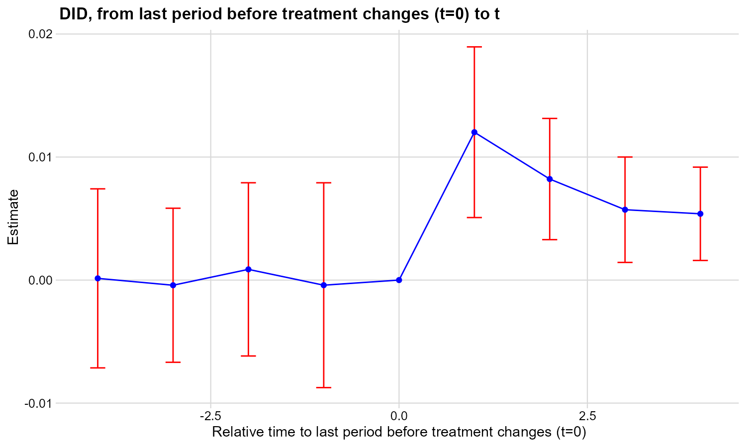
import pandas as pd
import polars as pl
import matplotlib.pyplot as plt
from did_multiplegt_dyn import DidMultiplegtDyn
df = pd.read_parquet("https://raw.githubusercontent.com/Credible-Answers/did_book/main/cc_xd_didtextbook_2025_9_30/Data%20sets/Gentzkow%20et%20al%202011/gentzkowetal_didtextbook.parquet")
df_pl = pl.from_pandas(df)
pd.set_option('display.float_format', lambda x: f'{x:.7f}')
gq6 = DidMultiplegtDyn(df=df_pl, outcome="prestout", group="cnty90",
    time="year", treatment="numdailies", effects=4, placebo=4,
    normalized=True, normalized_weights=True, effects_equal=True, cluster="cnty90")
gq6.fit(); gq6.summary()
gq6.plot()
plt.savefig("figures/ch08_fig82_normalized_es_Python.png", dpi=150, bbox_inches="tight")
Block Estimate SE LB CI UB CI N Switchers
Effect_1 0.0120186 0.0035392 0.0050818 0.0189554 5674 1119
Effect_2 0.0082126 0.0025136 0.0032860 0.0131392 4648 1054
Effect_3 0.0057192 0.0021857 0.0014353 0.0100031 3750 984
Effect_4 0.0053873 0.0019348 0.0015951 0.0091795 2980 917
Average_Total_Effect 0.0160565 0.0047761 0.0066956 0.0254174 8659 4074
Placebo_1 -0.0004159 0.0042471 -0.0087401 0.0079083 4471 902
Placebo_2 0.0008718 0.0035920 -0.0061704 0.0079140 2778 746
Placebo_3 -0.0004199 0.0031938 -0.0066796 0.0058398 1644 604
Placebo_4 0.0001390 0.0037130 -0.0071380 0.0074160 910 441
Joint nullity of effects : p = 0.006814
Joint nullity of placebos : p = 0.992198
Equality of effects : p = 0.165258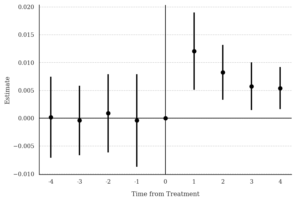
CQ#47: Interpreting the Normalized Effects
Interpret the previous results. Does it seem that the effect of lagged newspapers on turnout is larger or smaller than the effect of contemporaneous newspapers?
Normalized event-study and pre-trend estimates are shown in Figure 8.2. Normalized event-study estimates are decreasing with \(\ell\), but one cannot reject the null that all effects are equal (p-value = 0.17).
- \(w_{1,0} = 1\): the first event-study estimate is an effect of current newspapers on turnout.
- \(w_{2,0} = 0.48\) and \(w_{2,1} = 0.52\): the second normalized event-study estimate is an average of the effects of current and lagged newspapers, with approximately equal weights.
- \(w_{3,0} = 0.35\), \(w_{3,1} = 0.31\), and \(w_{3,2} = 0.33\): the third normalized event-study estimate is an average of the effects of current newspapers and of the first and second lag of newspapers, with approximately equal weights.
- \(w_{4,0} = 0.28\), \(w_{4,1} = 0.26\), \(w_{4,2} = 0.23\), and \(w_{4,3} = 0.24\): the fourth normalized event-study estimate is an average of the effects of current newspapers and of the first, second, and third lag of newspapers, again with approximately equal weights.
Then, as normalized event-study estimates and the weights assigned to the current number of newspapers are both decreasing with \(\ell\), lagged newspapers may have a smaller effect on turnout than current newspapers.
CQ#48: Joint Test of No Dynamic Effects
Restrict to counties whose treatment does not change between \(F_g\) and \(F_g + 1\), and test whether the first and second non-normalized effects are equal.
* ssc install did_multiplegt_dyn, replace
copy "https://raw.githubusercontent.com/Credible-Answers/did_book/main/cc_xd_didtextbook_2025_9_30/Data%20sets/Gentzkow%20et%20al%202011/gentzkowetal_didtextbook.dta" "gentzkowetal_didtextbook.dta", replace
use "gentzkowetal_didtextbook.dta", clear
did_multiplegt_dyn prestout cnty90 year numdailies if year<first_change | same_treat_after_first_change==1, effects(2) effects_equal(all) same_switchers graph_off
--------------------------------------------------------------------------------
Estimation of treatment effects: Event-study effects
--------------------------------------------------------------------------------
| Estimate SE LB CI UB CI N Switchers
-------------+------------------------------------------------------------------
Effect_1 | .01525 .0058956 .0036949 .0268052 5019 512
Effect_2 | .0164091 .0073633 .0019773 .0308409 4101 512
--------------------------------------------------------------------------------
Test of joint nullity of the effects : p-value = .0291303
Test of equality of the effects : p-value = .83016664
--------------------------------------------------------------------------------
Average cumulative (total) effect per treatment unit
--------------------------------------------------------------------------------
| Estimate SE LB CI UB CI N Switch x Periods
-------------+--------------------------------------------------------------------------
Av_tot_eff | .0138306 .0053281 .0033878 .0242734 5605 1024
--------------------------------------------------------------------------------
Average number of time periods over which a treatment's effect is accumulated = 1.5library(haven); library(DIDmultiplegtDYN)
load(url("https://raw.githubusercontent.com/Credible-Answers/did_book/main/cc_xd_didtextbook_2025_9_30/Data%20sets/Gentzkow%20et%20al%202011/gentzkowetal_didtextbook.RData"))
df_sub <- subset(df, year < first_change | same_treat_after_first_change == 1)
bonus <- did_multiplegt_dyn(
df = df_sub, outcome = "prestout", group = "cnty90",
time = "year", treatment = "numdailies",
effects = 2, effects_equal = TRUE,
same_switchers = TRUE, graph_off = TRUE)----------------------------------------------------------------------
Estimation of treatment effects: Event-study effects
----------------------------------------------------------------------
Estimate SE LB CI UB CI N Switchers
Effect_1 0.01525 0.00590 0.00369 0.02681 5,019 512
Effect_2 0.01641 0.00736 0.00198 0.03084 4,101 512
Test of joint nullity of the effects : p-value = 0.0291
Test of equality of the effects : p-value = 0.8302
----------------------------------------------------------------------
Average cumulative (total) effect per treatment unit
----------------------------------------------------------------------
Estimate SE LB CI UB CI N Switchers
0.01383 0.00533 0.00339 0.02427 5,605 1,024
Average number of time periods over which a treatment effect is accumulated: 1.5000import pandas as pd
import polars as pl
from did_multiplegt_dyn import DidMultiplegtDyn
df = pd.read_parquet("https://raw.githubusercontent.com/Credible-Answers/did_book/main/cc_xd_didtextbook_2025_9_30/Data%20sets/Gentzkow%20et%20al%202011/gentzkowetal_didtextbook.parquet")
df_sub = df[(df['year'] < df['first_change']) | (df['same_treat_after_first_change'] == 1)].copy()
df_pl = pl.from_pandas(df_sub)
bonus = DidMultiplegtDyn(df=df_pl, outcome="prestout", group="cnty90",
time="year", treatment="numdailies", effects=2,
same_switchers=True, effects_equal=True, cluster="cnty90")
bonus.fit(); bonus.summary()================================================================================
Estimation of treatment effects: Event-study effects
================================================================================
Block Estimate SE LB CI UB CI N Switchers N.w Switchers.w
Effect_1 0.015250 0.005896 0.003695 0.026805 5019.0 512.0 5019.0 512.0
Effect_2 0.016409 0.007363 0.001977 0.030841 4101.0 512.0 4101.0 512.0
Average_Total_Effect 0.013831 0.005328 0.003388 0.024273 5605.0 1024.0 5605.0 1024.0
Placebo_1 -0.001460 0.006378 -0.013961 0.011041 3936.0 413.0 3936.0 413.0
================================================================================
Test of joint nullity of the effects: p-value = 0.029130
Test of equality of the effects: p-value = 0.830167
The development of this package was funded by the European Union.
ERC REALLYCREDIBLE - GA N. 101043899Interpretation: In the subsample of 512 counties whose treatment does not change between \(F_g\) and \(F_g + 1\), the first and second event-study effects are very close (0.015 vs 0.016) and not significantly different (\(p = 0.83\)). This is consistent with the joint null that the first lag of newspapers does not affect turnout and that treatment effects are constant over time.
CQ#49: ATS and WATS Estimators (did_multiplegt_stat)
Using
did_multiplegt_stat, compute the ATS and WATS estimators withexact_matchand one placebo. Compare to the normalized event-study effects.
* ssc install did_multiplegt_stat, replace
copy "https://raw.githubusercontent.com/Credible-Answers/did_book/main/cc_xd_didtextbook_2025_9_30/Data%20sets/Gentzkow%20et%20al%202011/gentzkowetal_didtextbook.dta" "gentzkowetal_didtextbook.dta", replace
use "gentzkowetal_didtextbook.dta", clear
did_multiplegt_stat prestout cnty90 year numdailies, placebo(1) exact_match
-------------------------------------
N = 15466
Estimation method = Reg. Adjustment
Common Support = Exact Matching
-------------------------------------
----------------------------------------------------------------------
Average Slope (AS)
----------------------------------------------------------------------
Estimate SE LB CI UB CI Switchers Stayers
AS 0.0060678 0.0016463 0.002841 0.0092947 4423 11043
----------------------------------------------------------------------
Placebo(s) AS
----------------------------------------------------------------------
Estimate SE LB CI UB CI Switchers Stayers
AS -0.0011278 0.0025056 -0.0060387 0.0037832 2287 7743
----------------------------------------------------------------------
Weighted Average Slope (WAS)
----------------------------------------------------------------------
Estimate SE LB CI UB CI Switchers Stayers
WAS 0.0057351 0.0015079 0.0027796 0.0086905 4423 11043
----------------------------------------------------------------------
Placebo(s) WAS
----------------------------------------------------------------------
Estimate SE LB CI UB CI Switchers Stayers
WAS -0.0000123 0.0022931 -0.0045069 0.0044822 2287 7743
141 switchers dropped (baseline treatment not in stayers' support)
22 stayers dropped (baseline treatment not in switchers' support)# pip install did-multiplegt-stat
import pandas as pd
from did_multiplegt_stat import DIDMultiplegtStat
df = pd.read_parquet("https://raw.githubusercontent.com/Credible-Answers/did_book/main/cc_xd_didtextbook_2025_9_30/Data%20sets/Gentzkow%20et%20al%202011/gentzkowetal_didtextbook.parquet")
model = DIDMultiplegtStat(
estimator=["as", "was"],
order=1,
placebo=1,
exact_match=True,
asinstata=True,
)
model.fit(df, Y="prestout", ID="cnty90", Time="year", D="numdailies")
model.summary()N = 15466
WAS Method = Reg. Adjustment
Common Support = Exact Matching
-----------------------------------
----------------------------------------------------------------------
Estimation of AS
----------------------------------------------------------------------
Estimate SE LB CI UB CI Switchers Stayers
AS 0.0061145 0.0016266 0.0029263 0.0093027 4,423 11,043
----------------------------------------------------------------------
Placebo(s) AS
----------------------------------------------------------------------
Estimate SE LB CI UB CI Switchers Stayers
Placebo_1 -0.0011280 0.0025056 -0.0060389 0.0037829 2,287 7,743
----------------------------------------------------------------------
Estimation of WAS
----------------------------------------------------------------------
Estimate SE LB CI UB CI Switchers Stayers
WAS 0.0057750 0.0014865 0.0028614 0.0086885 4,423 11,043
----------------------------------------------------------------------
Placebo(s) WAS
----------------------------------------------------------------------
Estimate SE LB CI UB CI Switchers Stayers
Placebo_1 -0.0000125 0.0022931 -0.0045071 0.0044820 2,287 7,743Interpretation: The ATS (\(\approx 0.006\)) and WATS (\(\approx 0.006\)) are significant and positive. The placebo estimates are small and insignificant, supporting the parallel-trends assumption. These estimates are roughly half the magnitude of \(\widehat{AVSQ}^n_1 = 0.012\), which suggests a non-linear treatment response.