Chapter 6: Designs with Variation in Treatment Timing
Overview
Dataset: Wolfers (2006) — wolfers2006_didtextbook.dta(Stata), wolfers2006_didtextbook.RData (R), wolfers2006_didtextbook.parquet (Python)
This chapter analyzes the effect of unilateral divorce laws (UDL) on divorce rates using a binary-and-staggered design. Between 1968 and 1988, 29 US states adopted UDLs. The panel covers 51 states from 1956 to 1988, with population weights and state-clustered standard errors throughout.
Key topics: decomposition of the static TWFE estimator, event-study TWFE, and four heterogeneity-robust estimators (Sun & Abraham, Callaway & Sant’Anna, de Chaisemartin & D’Haultfœuille, Borusyak et al.).
PanelView
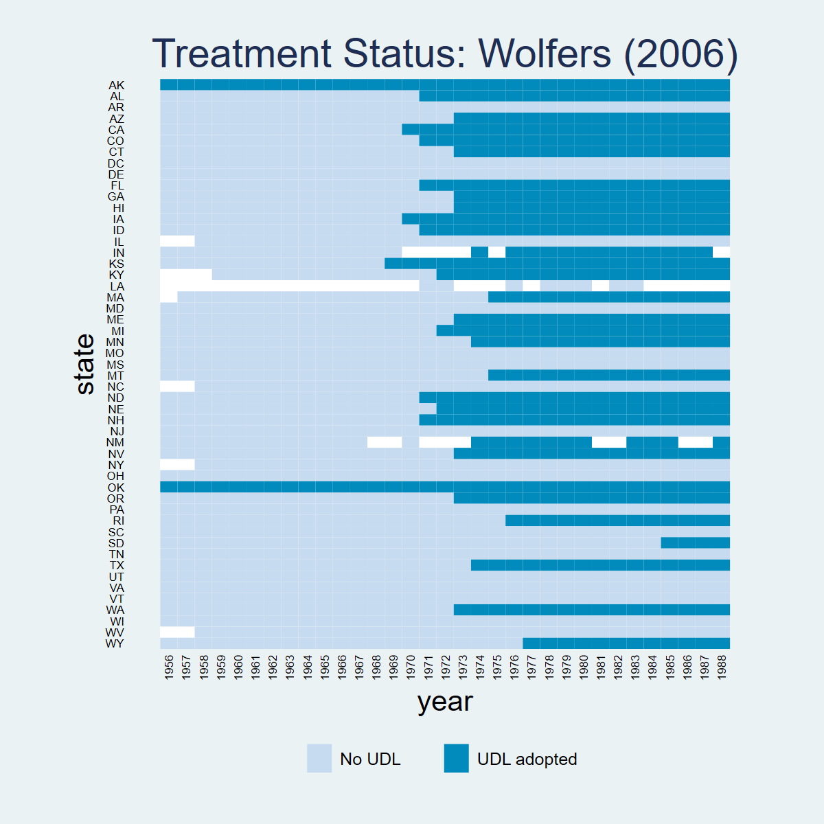
* ssc install panelview, replace
copy "https://raw.githubusercontent.com/Credible-Answers/did_book/main/cc_xd_didtextbook_2025_9_30/Data%20sets/Wolfers%202006/wolfers2006_didtextbook.dta" "wolfers2006_didtextbook.dta", replace
use "wolfers2006_didtextbook.dta", clear
panelview div_rate udl, i(state) t(year) type(treat) title("Treatment Status: Wolfers (2006)") legend(label(1 "No UDL") label(2 "UDL adopted"))library(panelView)
load(url("https://raw.githubusercontent.com/Credible-Answers/did_book/main/cc_xd_didtextbook_2025_9_30/Data%20sets/Wolfers%202006/wolfers2006_didtextbook.RData"))
df <- haven::zap_labels(df)
df <- as.data.frame(df)
p <- panelview(div_rate ~ udl, data = df, index = c("state", "year"), type = "treat",
main = "Wolfers (2006)", ylab = "")
print(p) # lo muestra en Plots
dir.create("figures", showWarnings = FALSE)
png("figures/ch06_panelview_R.png", width = 1000, height = 600)
print(p)
dev.off()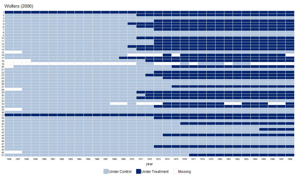
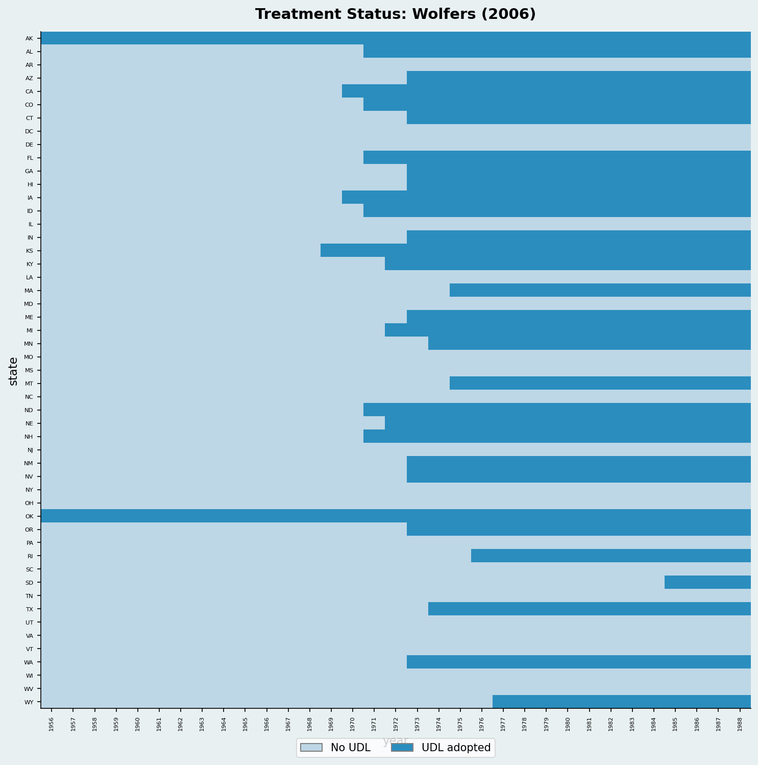
import pandas as pd
import matplotlib.pyplot as plt
import matplotlib.colors as mcolors
from matplotlib.patches import Patch
df = pd.read_parquet("https://raw.githubusercontent.com/Credible-Answers/did_book/main/cc_xd_didtextbook_2025_9_30/Data%20sets/Wolfers%202006/wolfers2006_didtextbook.parquet")
states_sorted = (df.groupby("state")["cohort"]
                 .first().sort_values(ascending=False).index)
state_idx = {s: i for i, s in enumerate(states_sorted)}
years = sorted(df["year"].unique())

fig, ax = plt.subplots(figsize=(14, 10))
cmap = mcolors.ListedColormap(["#4292C6", "#EF6548"])
for _, row in df.iterrows():
    si = state_idx[row["state"]]
    yi = years.index(row["year"])
    color = 1 if row["udl"] == 1 else 0
    ax.add_patch(plt.Rectangle((yi, si), 1, 1, color=cmap(color)))

ax.set_xlim(0, len(years)); ax.set_ylim(0, len(states_sorted))
ax.set_xticks(range(0, len(years), 5))
ax.set_xticklabels([str(int(years[i])) for i in range(0, len(years), 5)],
                    rotation=45, fontsize=7)
ax.set_yticks([i + 0.5 for i in range(len(states_sorted))])
ax.set_yticklabels(states_sorted, fontsize=6)
ax.set_xlabel("Year"); ax.set_ylabel("State")
ax.set_title("Treatment Status: Wolfers (2006)")
legend_elements = [Patch(facecolor="#4292C6", label="Control"),
                   Patch(facecolor="#EF6548", label="Treated")]
ax.legend(handles=legend_elements, loc="lower right")
plt.tight_layout()
plt.savefig(FIGDIR / "ch06_panelview_Python.png", dpi=150)
CQ#25: Static TWFE Regression
Run the static TWFE regression of
div_rateon state and year FEs and the UDL treatment, weighting by population and clustering at the state level. Do UDLs have an effect on divorces?
copy "https://raw.githubusercontent.com/Credible-Answers/did_book/main/cc_xd_didtextbook_2025_9_30/Data%20sets/Wolfers%202006/wolfers2006_didtextbook.dta" "wolfers2006_didtextbook.dta", replace
use "wolfers2006_didtextbook.dta", clear
reg div_rate udl i.state i.year [w=stpop], vce(cluster state)
Linear regression Number of obs = 1,631
R-squared = 0.9305
Root MSE = .52417
(Std. err. adjusted for 51 clusters in state)
------------------------------------------------------------------------------
| Robust
div_rate | Coefficient std. err. t P>|t| [95% conf. interval]
-------------+----------------------------------------------------------------
udl | -.0548378 .1507695 -0.36 0.718 -.3576673 .2479917
------------------------------------------------------------------------------library(haven); library(fixest)
load(url("https://raw.githubusercontent.com/Credible-Answers/did_book/main/cc_xd_didtextbook_2025_9_30/Data%20sets/Wolfers%202006/wolfers2006_didtextbook.RData"))
m1 <- feols(div_rate ~ udl + i(year) | state,
data = df, weights = ~stpop, cluster = ~state,
ssc = ssc(fixef.K = "full"))Variable Coefficient Std. err. t [95% Conf. Interval]
------------------------------------------------------------------------------------------
udl -0.0548378 0.1507695 -0.36 [ -0.3503461, 0.2406705]
N = 1631 | R-sq = 0.9305import pandas as pd
import pyfixest as pf
df = pd.read_parquet("https://raw.githubusercontent.com/Credible-Answers/did_book/main/cc_xd_didtextbook_2025_9_30/Data%20sets/Wolfers%202006/wolfers2006_didtextbook.parquet")
m1 = pf.feols('div_rate ~ udl + i(year) | state',
data=df, weights='stpop', vcov={'CRV1': 'state'},
ssc=pf.ssc(adj=True, fixef_k='full', cluster_adj=True))
m1.summary(digits=7)| Coefficient | Estimate | Std. Error | t value | Pr(>|t|) | 2.5% | 97.5% |
|:--------------|-----------:|-------------:|-----------:|-----------:|-----------:|-----------:|
| udl | -0.0548378 | 0.1507695 | -0.3637192 | 0.7176012 | -0.3576673 | 0.2479917 |
RMSE: 1031.4486884 R2: 0.9304837 R2 Within: 0.8298766 Interpretation: \(\hat{\beta}_{fe} = -0.055\) (s.e. = 0.15, p = 0.72). The coefficient is small and insignificant. According to this regression, UDLs do not affect divorce rates.
CQ#26: Decompose Static TWFE
Decompose \(\hat{\beta}_{fe}\) using
twowayfeweights. Does it estimate a convex combination of effects? Could it be biased for the ATT?
* ssc install twowayfeweights, replace
copy "https://raw.githubusercontent.com/Credible-Answers/did_book/main/cc_xd_didtextbook_2025_9_30/Data%20sets/Wolfers%202006/wolfers2006_didtextbook.dta" "wolfers2006_didtextbook.dta", replace
use "wolfers2006_didtextbook.dta", clear
twowayfeweights div_rate state year udl, type(feTR) test_random_weights(exposurelength) weight(stpop)
Under the common trends assumption,
the TWFE coefficient beta, equal to -0.0548, estimates a weighted sum of 522 ATTs.
490 ATTs receive a positive weight, and 32 receive a negative weight.
------------------------------------------------
Treat. var: udl # ATTs Σ weights
------------------------------------------------
Positive weights 490 1.0259
Negative weights 32 -0.0259
------------------------------------------------
Total 522 1.0000
------------------------------------------------
Regression of variables possibly correlated with the treatment effect on the weights
Coef SE t-stat Correlation
exposurele~h -8.2883613 .21360588 -38.80212 -.73253245library(haven); library(TwoWayFEWeights)
load(url("https://raw.githubusercontent.com/Credible-Answers/did_book/main/cc_xd_didtextbook_2025_9_30/Data%20sets/Wolfers%202006/wolfers2006_didtextbook.RData"))
decomp2 <- twowayfeweights(df, "div_rate", "state", "year", "udl",
type = "feTR",
test_random_weights = "exposurelength",
weights = df$stpop)Under the common trends assumption,
beta estimates a weighted sum of 522 ATTs.
490 ATTs receive a positive weight, and 32 receive a negative weight.
Treat. var: udl ATTs Σ weights
Positive weights 490 1.0259
Negative weights 32 -0.0259
Total 522 1
Regression:
Coef SE t-stat Correlation
RW_exposurelength -8.288361 0.2136059 -38.80212 -0.7325324import pandas as pd
from twowayfeweights import twowayfeweights
df = pd.read_parquet("https://raw.githubusercontent.com/Credible-Answers/did_book/main/cc_xd_didtextbook_2025_9_30/Data%20sets/Wolfers%202006/wolfers2006_didtextbook.parquet")
result = twowayfeweights(df, "div_rate", "state", "year", "udl",
type="feTR", weights="stpop",
test_random_weights="exposurelength")
print(result)Under the common trends assumption,
beta estimates a weighted sum of 522 ATTs.
490 ATTs receive a positive weight, and 32 receive a negative weight.
Sum of positive weights: 1.0259
Sum of negative weights: -0.0259
Regression of variables possibly correlated with the treatment effect on the weights
Coef SE t-stat Correlation
exposurelength -8.288361 0.213606 -38.8021 -0.732532Interpretation: Under parallel trends, \(\hat{\beta}_{fe}\) estimates a weighted sum of ATTs. The vast majority receive positive weights (sum ≈ 1.026) and 32 receive negative weights (sum ≈ −0.026), an “almost convex” combination. However, weights are strongly negatively correlated with exposure length (corr = −0.73, t = −38.8): \(\hat{\beta}_{fe}\) heavily downweights long-run effects. It could differ from the ATT if treatment effects vary with length of exposure.
CQ#27: Test Randomized Treatment Timing
Test whether pre-treatment outcomes differ across early, late, and never adopters (excluding always-treated states, restricting to years ≤ 1968).
copy "https://raw.githubusercontent.com/Credible-Answers/did_book/main/cc_xd_didtextbook_2025_9_30/Data%20sets/Wolfers%202006/wolfers2006_didtextbook.dta" "wolfers2006_didtextbook.dta", replace
use "wolfers2006_didtextbook.dta", clear
reg div_rate i.early_late_never if cohort!=1956 & year<=1968 [w=stpop], vce(cluster state)
Linear regression Number of obs = 611
F(2, 47) = 7.46
Prob > F = 0.0015
R-squared = 0.1707
(Std. err. adjusted for 48 clusters in state)
----------------------------------------------------------------------------------
| Robust
div_rate | Coefficient std. err. t P>|t| [95% conf. interval]
-----------------+----------------------------------------------------------------
early_late_never |
2 | -.0457088 .4927483 -0.09 0.926 -1.03699 .9455728
3 | -1.363398 .3751166 -3.63 0.001 -2.118035 -.608761
|
_cons | 3.054891 .2584305 11.82 0.000 2.534996 3.574786
----------------------------------------------------------------------------------library(haven)
library(dplyr)
load(url("https://raw.githubusercontent.com/Credible-Answers/did_book/main/cc_xd_didtextbook_2025_9_30/Data%20sets/Wolfers%202006/wolfers2006_didtextbook.RData"))
df3 <- df %>% filter(cohort != 1956, year <= 1968)
m3 <- feols(div_rate ~ i(early_late_never),
data = df3, weights = ~stpop, cluster = ~state,
ssc = ssc(fixef.K = "full"))Variable Coefficient Std. err. t [95% Conf. Interval]
------------------------------------------------------------------------------------------
(Intercept) 3.0548909 0.2584305 11.82 [ 2.5483670, 3.5614147]
early_late_never::2 -0.0457088 0.4927483 -0.09 [ -1.0114954, 0.9200777]
early_late_never::3 -1.3633981 0.3751166 -3.63 [ -2.0986266, -0.6281697]
N = 611 | R-sq = 0.1707import pandas as pd
import pyfixest as pf
import numpy as np
from scipy import stats
df = pd.read_parquet("https://raw.githubusercontent.com/Credible-Answers/did_book/main/cc_xd_didtextbook_2025_9_30/Data%20sets/Wolfers%202006/wolfers2006_didtextbook.parquet")
df3 = df[(df['cohort'] != 1956) & (df['year'] <= 1968)].copy()
m3 = pf.feols('div_rate ~ C(early_late_never)',
data=df3, weights='stpop', vcov={'CRV1': 'state'},
ssc=pf.ssc(adj=True, fixef_k='full', cluster_adj=True))
m3.summary(digits=7)
# Joint test: all early_late_never coefficients = 0
names = list(m3.coef().index)
tested = [n for n in names if n != "Intercept"]
idx = [names.index(n) for n in tested]
b = m3.coef().values[idx]
V = np.asarray(m3._vcov)[np.ix_(idx, idx)]
q = len(tested)
G = df3["state"].nunique()
F = float(b @ np.linalg.solve(V, b)) / q
p = stats.f.sf(F, q, G - 1)
print(f"\nF({q}, {G - 1}) = {F:.2f} Prob > F = {p:.4f}")| Coefficient | Estimate | Std. Error | t value | Pr(>|t|) | 2.5% | 97.5% |
|:---------------------------|-----------:|-------------:|-----------:|-----------:|-----------:|-----------:|
| Intercept | 3.0548909 | 0.2584305 | 11.8209361 | 0.0000000 | 2.5349957 | 3.5747861 |
| C(early_late_never)[T.2.0] | -0.0457088 | 0.4927483 | -0.0927630 | 0.9264861 | -1.0369904 | 0.9455728 |
| C(early_late_never)[T.3.0] | -1.3633981 | 0.3751166 | -3.6345987 | 0.0006881 | -2.1180353 | -0.6087610 |
---
RMSE: 2836.5163952 R2: 0.1707435
F(2, 48) = 7.46 Prob > F = 0.0015Interpretation: F-test p-value = 0.0015 — we reject that pre-treatment outcomes are the same across groups. Treatment timing is not randomly assigned: never-adopters have significantly lower divorce rates before any state adopts a UDL.
TWFE event-study graph
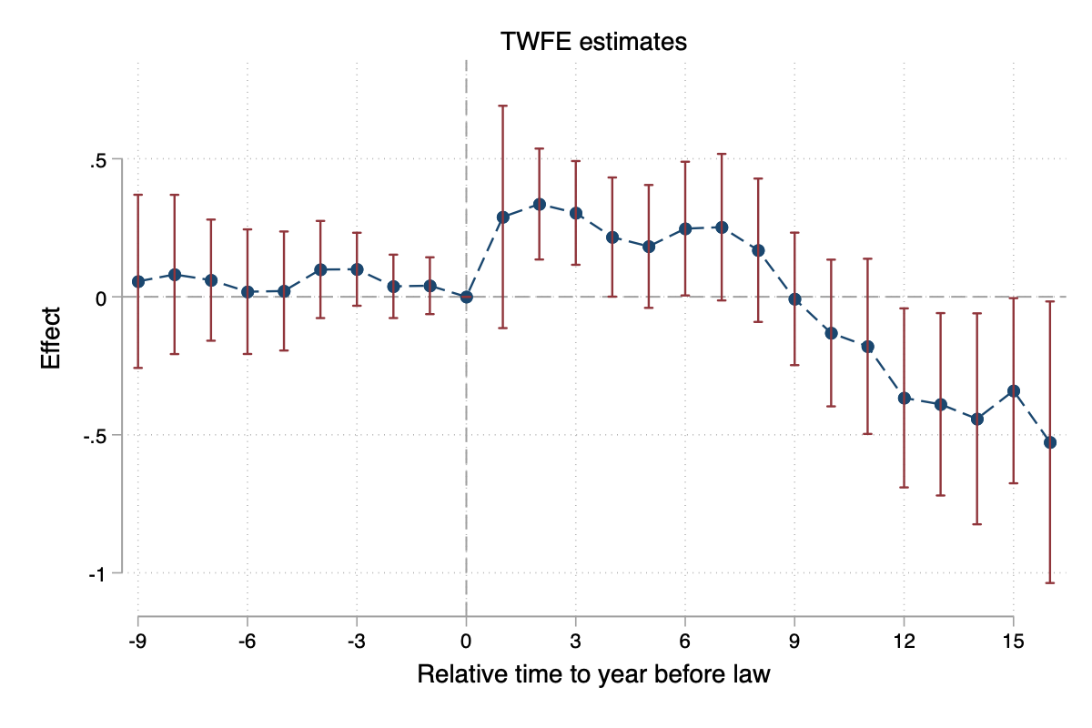
Let’s now depict Figure 6.2: the TWFE event-study estimates of the effect of unilateral divorce laws on the divorce rate, by years relative to the year before the law was passed. It shows the pre-period coefficients (rel_timeminus9–rel_timeminus1) and the post-period coefficients (rel_time1–rel_time16), with 95% confidence intervals. We will use this graph as input to answer CQ#28 and CQ#32 in detail.
copy "https://raw.githubusercontent.com/Credible-Answers/did_book/main/cc_xd_didtextbook_2025_9_30/Data%20sets/Wolfers%202006/wolfers2006_didtextbook.dta" "wolfers2006_didtextbook.dta", replace
use "wolfers2006_didtextbook.dta", clear
* Run the regression
reg div_rate rel_time* i.state i.year [w=stpop], vce(cluster state)

* Pull coefficients and CIs into a postfile
tempname pf
tempfile coefs
postfile `pf' rel_time coef ci_lo ci_hi using `coefs'

* Post-period coefficients: rel_time1 ... rel_time16
forvalues t = 1/16 {
    local b  = _b[rel_time`t']
    local se = _se[rel_time`t']
    local lo = `b' - 1.96 * `se'
    local hi = `b' + 1.96 * `se'
    post `pf' (`t') (`b') (`lo') (`hi')
}

* Pre-period coefficients: rel_timeminus1 ... rel_timeminus9 (negative event time)
forvalues t = 1/9 {
    local b  = _b[rel_timeminus`t']
    local se = _se[rel_timeminus`t']
    local lo = `b' - 1.96 * `se'
    local hi = `b' + 1.96 * `se'
    post `pf' (-`t') (`b') (`lo') (`hi')
}

* Add the reference period (rel_time = 0) as a zero point
post `pf' (0) (0) (0) (0)

postclose `pf'

* Load the coefficient dataset
preserve
use `coefs', clear
sort rel_time

* Plot
twoway (scatter coef rel_time, msize(medlarge) msymbol(o) mcolor(navy) legend(off)) ///
       (line coef rel_time, lcolor(navy)) ///
       (rcap ci_hi ci_lo rel_time, lcolor(maroon)), ///
       title("TWFE estimates") ///
       xtitle("Relative time to year before law") ///
       ytitle("Effect") ///
       ylabel(-1(.5)0.5) yscale(range(-1.1 0.8)) ///
       xlabel(-9(3)15) ///
       xline(0, lcolor(gs10) lpattern(dash)) ///
       yline(0, lcolor(gs10) lpattern(dash)) ///
       legend(off)

graph export "figures/ch06_fig62_twfe_es.png", replace width(1200)
restore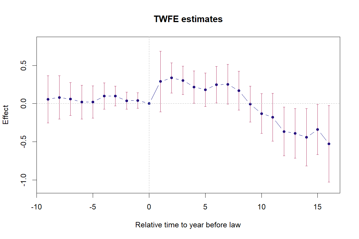
library(haven)
load(url("https://raw.githubusercontent.com/Credible-Answers/did_book/main/cc_xd_didtextbook_2025_9_30/Data%20sets/Wolfers%202006/wolfers2006_didtextbook.RData"))
es_coefs <- data.frame(
    rel_time = c(-(9:1), 0, 1:16),
    coef = c(coef(m4)[paste0("rel_timeminus", 9:1)], 0,
             coef(m4)[paste0("rel_time", 1:16)]),
    se = c(se(m4)[paste0("rel_timeminus", 9:1)], 0,
           se(m4)[paste0("rel_time", 1:16)]))
es_coefs$ci_lo <- es_coefs$coef - 1.96 * es_coefs$se
es_coefs$ci_hi <- es_coefs$coef + 1.96 * es_coefs$se

plot(es_coefs$rel_time, es_coefs$coef, type = "b", pch = 19, col = "navy",
     xlab = "Relative time to year before law", ylab = "Effect",
     main = "TWFE estimates", ylim = c(-1.1, 0.8), xlim = c(-9, 16))
arrows(es_coefs$rel_time, es_coefs$ci_lo, es_coefs$rel_time, es_coefs$ci_hi,
       length = 0.03, angle = 90, code = 3, col = "maroon")
abline(h = 0, lty = 2, col = "gray60"); abline(v = 0, lty = 2, col = "gray60")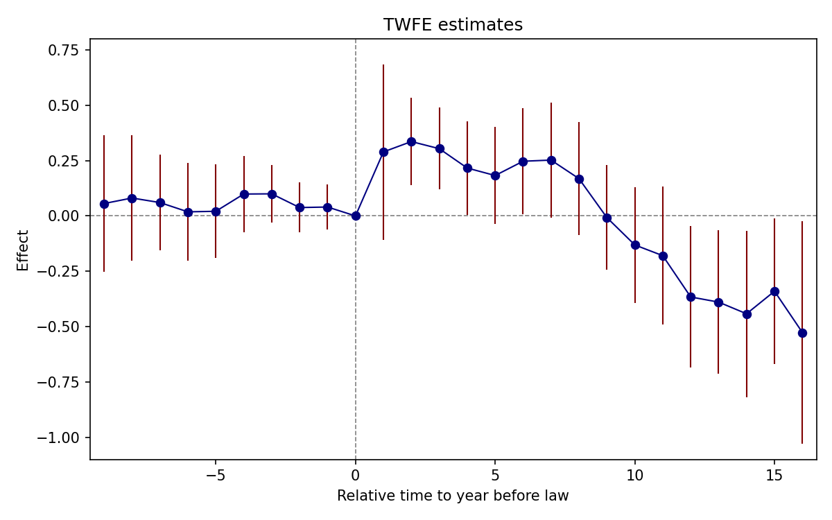
import pandas as pd
import pyfixest as pf
import matplotlib.pyplot as plt
from pathlib import Path

df = pd.read_parquet("https://raw.githubusercontent.com/Credible-Answers/did_book/main/cc_xd_didtextbook_2025_9_30/Data%20sets/Wolfers%202006/wolfers2006_didtextbook.parquet")

rt_pos = [f"rel_time{i}" for i in range(1, 17)]
rt_neg = [f"rel_timeminus{i}" for i in range(9, 0, -1)]
fml = "div_rate ~ " + " + ".join(rt_pos + rt_neg) + " + i(year) | state"
m4 = pf.feols(fml, data=df, weights="stpop", vcov={"CRV1": "state"},
              ssc=pf.ssc(adj=True, fixef_k="full", cluster_adj=True))

rt = list(range(-9, 0)) + [0] + list(range(1, 17))
names = rt_neg + [None] + rt_pos
coefs = [m4.coef()[n] if n else 0.0 for n in names]
ses = [m4.se()[n] if n else 0.0 for n in names]

fig, ax = plt.subplots(figsize=(10, 6))
ax.errorbar(rt, coefs, yerr=[1.96 * s for s in ses], fmt='o-', color='navy',
            ecolor='maroon', capsize=3, markersize=5)
ax.axhline(0, color='gray', linestyle='--')
ax.axvline(0, color='gray', linestyle='--')
ax.set_xticks(range(-9, 16, 5))
ax.set_ylim(-1.1, 0.8)
ax.set_xlabel("Relative time to year before law")
ax.set_ylabel("Effect")
ax.set_title("TWFE estimates")
plt.tight_layout()
Path("figures").mkdir(exist_ok=True)
plt.savefig("figures/ch06_fig62_twfe_es_Python.png", dpi=150)
CQ#28: Event-Study TWFE Regression
Run the event-study TWFE regression with
rel_timeindicators. Test pre-trends jointly.
copy "https://raw.githubusercontent.com/Credible-Answers/did_book/main/cc_xd_didtextbook_2025_9_30/Data%20sets/Wolfers%202006/wolfers2006_didtextbook.dta" "wolfers2006_didtextbook.dta", replace
use "wolfers2006_didtextbook.dta", clear
reg div_rate rel_time* i.state i.year [w=stpop], vce(cluster state)
test rel_timeminus1 rel_timeminus2 rel_timeminus3 rel_timeminus4 rel_timeminus5 rel_timeminus6 rel_timeminus7 rel_timeminus8 rel_timeminus9
(Std. err. adjusted for 51 clusters in state)
--------------------------------------------------------------------------------
| Robust
div_rate | Coefficient std. err. t P>|t| [95% conf. interval]
---------------+----------------------------------------------------------------
rel_time1 | .2891561 .2054259 1.41 0.165 -.1234539 .7017661
rel_time2 | .3358503 .1024966 3.28 0.002 .1299798 .5417208
rel_time3 | .3037197 .0958368 3.17 0.003 .1112258 .4962136
rel_time4 | .2162947 .1100871 1.96 0.055 -.0048218 .4374112
rel_time5 | .1824478 .1135503 1.61 0.114 -.0456248 .4105203
rel_time6 | .2469589 .1235802 2.00 0.051 -.0012592 .4951769
rel_time7 | .2521922 .1354015 1.86 0.068 -.0197698 .5241541
rel_time8 | .1684823 .1324744 1.27 0.209 -.0976004 .434565
rel_time9 | -.007686 .1224421 -0.06 0.950 -.2536183 .2382463
rel_time10 | -.1312296 .135582 -0.97 0.338 -.4035541 .1410948
rel_time11 | -.1795675 .1618587 -1.11 0.273 -.5046704 .1455353
rel_time12 | -.3662379 .165442 -2.21 0.031 -.698538 -.0339379
rel_time13 | -.3894262 .1685244 -2.31 0.025 -.7279175 -.0509349
rel_time14 | -.4421197 .1949527 -2.27 0.028 -.8336937 -.0505457
rel_time15 | -.3402803 .1710816 -1.99 0.052 -.6839078 .0033472
rel_time16 | -.526895 .2602054 -2.02 0.048 -1.049533 -.0042572
rel_timeminus1 | .0401147 .0525088 0.76 0.448 -.0653522 .1455817
rel_timeminus2 | .0377587 .058556 0.64 0.522 -.0798546 .1553719
rel_timeminus3 | .0997316 .0674681 1.48 0.146 -.0357821 .2352453
rel_timeminus4 | .0988424 .0897758 1.10 0.276 -.0814777 .2791625
rel_timeminus5 | .020862 .1099841 0.19 0.850 -.2000476 .2417716
rel_timeminus6 | .0183927 .1151678 0.16 0.874 -.2129287 .2497141
rel_timeminus7 | .0602846 .1119554 0.54 0.593 -.1645845 .2851537
rel_timeminus8 | .0808726 .1471298 0.55 0.585 -.2146462 .3763915
rel_timeminus9 | .0558855 .1600016 0.35 0.728 -.2654871 .3772581
---------------+----------------------------------------------------------------
F( 9, 50) = 0.51
Prob > F = 0.8631library(fixest)
library(haven)
load(url("https://raw.githubusercontent.com/Credible-Answers/did_book/main/cc_xd_didtextbook_2025_9_30/Data%20sets/Wolfers%202006/wolfers2006_didtextbook.RData"))
df <- as.data.frame(zap_labels(df))
rel_time_vars <- names(df)[grepl("^rel_time", names(df))]
rel_time_formula <- paste("div_rate ~", paste(rel_time_vars, collapse = " + "),
"+ i(state) + i(year)")
event_study_twfe <- feols(as.formula(rel_time_formula), data = df,
weights = ~stpop, cluster = ~state)
wald(event_study_twfe, keep = "rel_timeminus")Variable Coefficient Std. err. t [95% Conf. Interval]
------------------------------------------------------------------------------------------
rel_time1 0.2891561 0.2054259 1.41 [ -0.1134786, 0.6917908]
rel_time2 0.3358503 0.1024966 3.28 [ 0.1349569, 0.5367437]
rel_time3 0.3037197 0.0958368 3.17 [ 0.1158795, 0.4915599]
rel_time4 0.2162947 0.1100871 1.96 [ 0.0005240, 0.4320654]
rel_time5 0.1824478 0.1135503 1.61 [ -0.0401109, 0.4050064]
rel_time6 0.2469589 0.1235802 2.00 [ 0.0047418, 0.4891760]
rel_time7 0.2521922 0.1354015 1.86 [ -0.0131948, 0.5175791]
rel_time8 0.1684823 0.1324744 1.27 [ -0.0911675, 0.4281321]
rel_time9 -0.0076860 0.1224421 -0.06 [ -0.2476726, 0.2323006]
rel_time10 -0.1312296 0.1355820 -0.97 [ -0.3969703, 0.1345111]
rel_time11 -0.1795675 0.1618587 -1.11 [ -0.4968107, 0.1376756]
rel_time12 -0.3662379 0.1654420 -2.21 [ -0.6905043, -0.0419716]
rel_time13 -0.3894262 0.1685244 -2.31 [ -0.7197342, -0.0591183]
rel_time14 -0.4421197 0.1949527 -2.27 [ -0.8242270, -0.0600124]
rel_time15 -0.3402803 0.1710816 -1.99 [ -0.6756002, -0.0049604]
rel_time16 -0.5268950 0.2602054 -2.02 [ -1.0368975, -0.0168925]
rel_timeminus1 0.0401147 0.0525088 0.76 [ -0.0628025, 0.1430319]
rel_timeminus2 0.0377587 0.0585560 0.64 [ -0.0770112, 0.1525285]
rel_timeminus3 0.0997316 0.0674681 1.48 [ -0.0325059, 0.2319691]
rel_timeminus4 0.0988424 0.0897758 1.10 [ -0.0771182, 0.2748030]
rel_timeminus5 0.0208620 0.1099841 0.19 [ -0.1947069, 0.2364309]
rel_timeminus6 0.0183927 0.1151678 0.16 [ -0.2073362, 0.2441217]
rel_timeminus7 0.0602846 0.1119554 0.54 [ -0.1591481, 0.2797173]
rel_timeminus8 0.0808726 0.1471298 0.55 [ -0.2075017, 0.3692470]
rel_timeminus9 0.0558855 0.1600016 0.35 [ -0.2577175, 0.3694885]
N = 1631 | R-sq = 0.9351
Wald test: stat = 0.506103, p-value = 0.870968, on 9 and 1,523 DoFimport pandas as pd
import pyfixest as pf
import numpy as np
from scipy import stats
df = pd.read_parquet("https://raw.githubusercontent.com/Credible-Answers/did_book/main/cc_xd_didtextbook_2025_9_30/Data%20sets/Wolfers%202006/wolfers2006_didtextbook.parquet")
rt_pos = [c for c in df.columns if c.startswith("rel_time") and "minus" not in c]
rt_neg = [c for c in df.columns if "rel_timeminus" in c]
fml = "div_rate ~ " + " + ".join(rt_pos + rt_neg) + " + i(year) | state"
m4 = pf.feols(fml, data=df, weights='stpop', vcov={'CRV1': 'state'},
ssc=pf.ssc(adj=True, fixef_k='full', cluster_adj=True))
m4.summary(digits=7)
# Joint test of the pre-trends: rel_timeminus1 = ... = rel_timeminus9 = 0
tested = [f"rel_timeminus{i}" for i in range(1, 10)]
names = list(m4.coef().index)
idx = [names.index(n) for n in tested]
b = m4.coef().values[idx]
V = np.asarray(m4._vcov)[np.ix_(idx, idx)]
q = len(tested)
G = df["state"].nunique()
F = float(b @ np.linalg.solve(V, b)) / q
p = stats.f.sf(F, q, G - 1)
print(f"\nF({q}, {G - 1}) = {F:.2f} Prob > F = {p:.4f}")| Coefficient | Estimate | Std. Error | t value | Pr(>|t|) | 2.5% | 97.5% |
|:---------------|-----------:|-------------:|-----------:|-----------:|-----------:|-----------:|
| rel_time1 | 0.2891561 | 0.2054259 | 1.4075935 | 0.1654383 | -0.1234539 | 0.7017661 |
| rel_time2 | 0.3358503 | 0.1024966 | 3.2766963 | 0.0019131 | 0.1299798 | 0.5417208 |
| rel_time3 | 0.3037197 | 0.0958368 | 3.1691339 | 0.0026089 | 0.1112258 | 0.4962136 |
| rel_time4 | 0.2162947 | 0.1100871 | 1.9647595 | 0.0550112 | -0.0048218 | 0.4374112 |
| rel_time5 | 0.1824478 | 0.1135503 | 1.6067569 | 0.1144054 | -0.0456248 | 0.4105203 |
| rel_time6 | 0.2469589 | 0.1235802 | 1.9983700 | 0.0511292 | -0.0012592 | 0.4951769 |
| rel_time7 | 0.2521922 | 0.1354015 | 1.8625505 | 0.0684062 | -0.0197698 | 0.5241541 |
| rel_time8 | 0.1684823 | 0.1324744 | 1.2718102 | 0.2093244 | -0.0976004 | 0.4345650 |
| rel_time9 | -0.0076860 | 0.1224421 | -0.0627724 | 0.9501980 | -0.2536183 | 0.2382463 |
| rel_time10 | -0.1312296 | 0.1355820 | -0.9678986 | 0.3377537 | -0.4035541 | 0.1410948 |
| rel_time11 | -0.1795675 | 0.1618587 | -1.1094090 | 0.2725613 | -0.5046704 | 0.1455353 |
| rel_time12 | -0.3662379 | 0.1654420 | -2.2136937 | 0.0314401 | -0.6985380 | -0.0339379 |
| rel_time13 | -0.3894262 | 0.1685244 | -2.3107998 | 0.0250068 | -0.7279175 | -0.0509349 |
| rel_time14 | -0.4421197 | 0.1949527 | -2.2678308 | 0.0276929 | -0.8336937 | -0.0505457 |
| rel_time15 | -0.3402803 | 0.1710816 | -1.9889943 | 0.0521876 | -0.6839078 | 0.0033472 |
| rel_time16 | -0.5268950 | 0.2602054 | -2.0249201 | 0.0482319 | -1.0495329 | -0.0042572 |
| rel_timeminus1 | 0.0401147 | 0.0525088 | 0.7639626 | 0.4484798 | -0.0653522 | 0.1455817 |
| rel_timeminus2 | 0.0377587 | 0.0585560 | 0.6448295 | 0.5219854 | -0.0798546 | 0.1553719 |
| rel_timeminus3 | 0.0997316 | 0.0674681 | 1.4782031 | 0.1456257 | -0.0357821 | 0.2352453 |
| rel_timeminus4 | 0.0988424 | 0.0897758 | 1.1009911 | 0.2761727 | -0.0814777 | 0.2791625 |
| rel_timeminus5 | 0.0208620 | 0.1099841 | 0.1896817 | 0.8503265 | -0.2000476 | 0.2417716 |
| rel_timeminus6 | 0.0183927 | 0.1151678 | 0.1597037 | 0.8737579 | -0.2129287 | 0.2497141 |
| rel_timeminus7 | 0.0602846 | 0.1119554 | 0.5384695 | 0.5926422 | -0.1645845 | 0.2851537 |
| rel_timeminus8 | 0.0808726 | 0.1471298 | 0.5496688 | 0.5849935 | -0.2146462 | 0.3763915 |
| rel_timeminus9 | 0.0558855 | 0.1600016 | 0.3492810 | 0.7283452 | -0.2654871 | 0.3772581 |
---
RMSE: 996.6048219 R2: 0.9351011 R2 Within: 0.8411765
F(9, 50) = 0.51 Prob > F = 0.8631Interpretation: Pre-trends are individually and jointly insignificant (F(9, 50) = 0.51, p = 0.86). Post-treatment effects are positive for the first ~8 years, then turn negative after year 9.
CQ#29: Decompose \(\hat{\beta}_1^{fe}\)
Use
twowayfeweightsto decompose \(\hat{\beta}_1^{fe}\), and compute the correlation between the weights and theyearvariable.
* ssc install twowayfeweights, replace
copy "https://raw.githubusercontent.com/Credible-Answers/did_book/main/cc_xd_didtextbook_2025_9_30/Data%20sets/Wolfers%202006/wolfers2006_didtextbook.dta" "wolfers2006_didtextbook.dta", replace
use "wolfers2006_didtextbook.dta", clear
twowayfeweights div_rate state year rel_time1, type(feTR) test_random_weights(year) weight(stpop) other_treatments(rel_time2-rel_time16) controls(rel_timeminus1-rel_timeminus9)
Under the common trends assumption,
the TWFE coefficient beta, equal to 0.2892, estimates the sum of several terms.
The first term is a weighted sum of 27 ATTs of the treatment.
27 ATTs receive a positive weight, and 0 receive a negative weight.
------------------------------------------------
Treat. var: rel_time1 # ATTs Σ weights
------------------------------------------------
Positive weights 27 1.0000
Negative weights 0 0.0000
------------------------------------------------
Total 27 1.0000
------------------------------------------------
The next term is a weighted sum of 29 ATTs of treatment 1 included in the other_treatments option.
16 ATTs receive a positive weight, and 13 receive a negative weight.
------------------------------------------------
Other treat.: rel_time2 # ATTs Σ weights
------------------------------------------------
Positive weights 16 0.0119
Negative weights 13 -0.0119
------------------------------------------------
Total 29 -0.0000
------------------------------------------------
The next term is a weighted sum of 28 ATTs of treatment 2 included in the other_treatments option.
10 ATTs receive a positive weight, and 18 receive a negative weight.
------------------------------------------------
Other treat.: rel_time3 # ATTs Σ weights
------------------------------------------------
Positive weights 10 0.0102
Negative weights 18 -0.0102
------------------------------------------------
Total 28 0.0000
------------------------------------------------
The next term is a weighted sum of 30 ATTs of treatment 3 included in the other_treatments option.
21 ATTs receive a positive weight, and 9 receive a negative weight.
------------------------------------------------
Other treat.: rel_time4 # ATTs Σ weights
------------------------------------------------
Positive weights 21 0.0083
Negative weights 9 -0.0083
------------------------------------------------
Total 30 0.0000
------------------------------------------------
The next term is a weighted sum of 29 ATTs of treatment 4 included in the other_treatments option.
21 ATTs receive a positive weight, and 8 receive a negative weight.
------------------------------------------------
Other treat.: rel_time5 # ATTs Σ weights
------------------------------------------------
Positive weights 21 0.0105
Negative weights 8 -0.0105
------------------------------------------------
Total 29 -0.0000
------------------------------------------------
The next term is a weighted sum of 29 ATTs of treatment 5 included in the other_treatments option.
26 ATTs receive a positive weight, and 3 receive a negative weight.
------------------------------------------------
Other treat.: rel_time6 # ATTs Σ weights
------------------------------------------------
Positive weights 26 0.0065
Negative weights 3 -0.0065
------------------------------------------------
Total 29 0.0000
------------------------------------------------
The next term is a weighted sum of 29 ATTs of treatment 6 included in the other_treatments option.
19 ATTs receive a positive weight, and 10 receive a negative weight.
------------------------------------------------
Other treat.: rel_time7 # ATTs Σ weights
------------------------------------------------
Positive weights 19 0.0023
Negative weights 10 -0.0023
------------------------------------------------
Total 29 0.0000
------------------------------------------------
The next term is a weighted sum of 29 ATTs of treatment 7 included in the other_treatments option.
19 ATTs receive a positive weight, and 10 receive a negative weight.
------------------------------------------------
Other treat.: rel_time8 # ATTs Σ weights
------------------------------------------------
Positive weights 19 0.0017
Negative weights 10 -0.0017
------------------------------------------------
Total 29 0.0000
------------------------------------------------
The next term is a weighted sum of 28 ATTs of treatment 8 included in the other_treatments option.
17 ATTs receive a positive weight, and 11 receive a negative weight.
------------------------------------------------
Other treat.: rel_time9 # ATTs Σ weights
------------------------------------------------
Positive weights 17 0.0011
Negative weights 11 -0.0011
------------------------------------------------
Total 28 0.0000
------------------------------------------------
The next term is a weighted sum of 28 ATTs of treatment 9 included in the other_treatments option.
14 ATTs receive a positive weight, and 14 receive a negative weight.
------------------------------------------------
Other treat.: rel_time10# ATTs Σ weights
------------------------------------------------
Positive weights 14 0.0009
Negative weights 14 -0.0009
------------------------------------------------
Total 28 0.0000
------------------------------------------------
The next term is a weighted sum of 29 ATTs of treatment 10 included in the other_treatments option.
13 ATTs receive a positive weight, and 16 receive a negative weight.
------------------------------------------------
Other treat.: rel_time11# ATTs Σ weights
------------------------------------------------
Positive weights 13 0.0009
Negative weights 16 -0.0009
------------------------------------------------
Total 29 0.0000
------------------------------------------------
The next term is a weighted sum of 29 ATTs of treatment 11 included in the other_treatments option.
17 ATTs receive a positive weight, and 12 receive a negative weight.
------------------------------------------------
Other treat.: rel_time12# ATTs Σ weights
------------------------------------------------
Positive weights 17 0.0010
Negative weights 12 -0.0010
------------------------------------------------
Total 29 0.0000
------------------------------------------------
The next term is a weighted sum of 28 ATTs of treatment 12 included in the other_treatments option.
17 ATTs receive a positive weight, and 11 receive a negative weight.
------------------------------------------------
Other treat.: rel_time13# ATTs Σ weights
------------------------------------------------
Positive weights 17 0.0010
Negative weights 11 -0.0010
------------------------------------------------
Total 28 0.0000
------------------------------------------------
The next term is a weighted sum of 26 ATTs of treatment 13 included in the other_treatments option.
13 ATTs receive a positive weight, and 13 receive a negative weight.
------------------------------------------------
Other treat.: rel_time14# ATTs Σ weights
------------------------------------------------
Positive weights 13 0.0007
Negative weights 13 -0.0007
------------------------------------------------
Total 26 0.0000
------------------------------------------------
The next term is a weighted sum of 24 ATTs of treatment 14 included in the other_treatments option.
11 ATTs receive a positive weight, and 13 receive a negative weight.
------------------------------------------------
Other treat.: rel_time15# ATTs Σ weights
------------------------------------------------
Positive weights 11 0.0012
Negative weights 13 -0.0012
------------------------------------------------
Total 24 0.0000
------------------------------------------------
The next term is a weighted sum of 100 ATTs of treatment 15 included in the other_treatments option.
65 ATTs receive a positive weight, and 35 receive a negative weight.
------------------------------------------------
Other treat.: rel_time16# ATTs Σ weights
------------------------------------------------
Positive weights 65 0.0068
Negative weights 35 -0.0068
------------------------------------------------
Total 100 0.0000
------------------------------------------------
Regression of variables on the weights attached to the treatment
Coef SE t-stat Correlation
year -15.333901 13.428752 -1.1418709 -.23224592library(haven); library(TwoWayFEWeights)
load(url("https://raw.githubusercontent.com/Credible-Answers/did_book/main/cc_xd_didtextbook_2025_9_30/Data%20sets/Wolfers%202006/wolfers2006_didtextbook.RData"))
rel_time_vars <- names(df)[grepl("^rel_time", names(df))]
other_rel_times <- rel_time_vars[rel_time_vars != "rel_time1"]
other_treatments <- other_rel_times[grepl("^rel_time[2-9]$|^rel_time1[0-6]$", other_rel_times)]
controls <- other_rel_times[grepl("minus", other_rel_times)]
decomp5 <- twowayfeweights(df, "div_rate", "state", "year", "rel_time1",
type = "feTR", test_random_weights = "year",
weights = df$stpop,
other_treatments = other_treatments,
controls = controls)Under the common trends assumption,
the TWFE coefficient beta, equal to 0.2892, estimates the sum of several terms.
The first term is a weighted sum of 27 ATTs.
27 ATTs receive a positive weight, and 0 receive a negative weight.
──────────────────────────────────────────
Treat. var: rel_time1 ATTs Σ weights
──────────────────────────────────────────
Positive weights 27 1
Negative weights 0 0
──────────────────────────────────────────
Total 27 1
──────────────────────────────────────────
The next term is a weighted sum of 29 ATTs.
16 ATTs receive a positive weight, and 13 receive a negative weight.
────────────────────────────────────────────
Other treat.: rel_time2 ATTs Σ weights
────────────────────────────────────────────
Positive weights 16 0.0119
Negative weights 13 -0.0119
────────────────────────────────────────────
Total 29 0
────────────────────────────────────────────
The next term is a weighted sum of 28 ATTs.
10 ATTs receive a positive weight, and 18 receive a negative weight.
────────────────────────────────────────────
Other treat.: rel_time3 ATTs Σ weights
────────────────────────────────────────────
Positive weights 10 0.0102
Negative weights 18 -0.0102
────────────────────────────────────────────
Total 28 0
────────────────────────────────────────────
The next term is a weighted sum of 30 ATTs.
21 ATTs receive a positive weight, and 9 receive a negative weight.
────────────────────────────────────────────
Other treat.: rel_time4 ATTs Σ weights
────────────────────────────────────────────
Positive weights 21 0.0083
Negative weights 9 -0.0083
────────────────────────────────────────────
Total 30 0
────────────────────────────────────────────
The next term is a weighted sum of 29 ATTs.
21 ATTs receive a positive weight, and 8 receive a negative weight.
────────────────────────────────────────────
Other treat.: rel_time5 ATTs Σ weights
────────────────────────────────────────────
Positive weights 21 0.0105
Negative weights 8 -0.0105
────────────────────────────────────────────
Total 29 0
────────────────────────────────────────────
The next term is a weighted sum of 29 ATTs.
26 ATTs receive a positive weight, and 3 receive a negative weight.
────────────────────────────────────────────
Other treat.: rel_time6 ATTs Σ weights
────────────────────────────────────────────
Positive weights 26 0.0065
Negative weights 3 -0.0065
────────────────────────────────────────────
Total 29 0
────────────────────────────────────────────
The next term is a weighted sum of 29 ATTs.
19 ATTs receive a positive weight, and 10 receive a negative weight.
────────────────────────────────────────────
Other treat.: rel_time7 ATTs Σ weights
────────────────────────────────────────────
Positive weights 19 0.0023
Negative weights 10 -0.0023
────────────────────────────────────────────
Total 29 0
────────────────────────────────────────────
The next term is a weighted sum of 29 ATTs.
19 ATTs receive a positive weight, and 10 receive a negative weight.
────────────────────────────────────────────
Other treat.: rel_time8 ATTs Σ weights
────────────────────────────────────────────
Positive weights 19 0.0017
Negative weights 10 -0.0017
────────────────────────────────────────────
Total 29 0
────────────────────────────────────────────
The next term is a weighted sum of 28 ATTs.
17 ATTs receive a positive weight, and 11 receive a negative weight.
────────────────────────────────────────────
Other treat.: rel_time9 ATTs Σ weights
────────────────────────────────────────────
Positive weights 17 0.0011
Negative weights 11 -0.0011
────────────────────────────────────────────
Total 28 0
────────────────────────────────────────────
The next term is a weighted sum of 28 ATTs.
14 ATTs receive a positive weight, and 14 receive a negative weight.
─────────────────────────────────────────────
Other treat.: rel_time10 ATTs Σ weights
─────────────────────────────────────────────
Positive weights 14 9e-04
Negative weights 14 -9e-04
─────────────────────────────────────────────
Total 28 0
─────────────────────────────────────────────
The next term is a weighted sum of 29 ATTs.
13 ATTs receive a positive weight, and 16 receive a negative weight.
─────────────────────────────────────────────
Other treat.: rel_time11 ATTs Σ weights
─────────────────────────────────────────────
Positive weights 13 9e-04
Negative weights 16 -9e-04
─────────────────────────────────────────────
Total 29 0
─────────────────────────────────────────────
The next term is a weighted sum of 29 ATTs.
17 ATTs receive a positive weight, and 12 receive a negative weight.
─────────────────────────────────────────────
Other treat.: rel_time12 ATTs Σ weights
─────────────────────────────────────────────
Positive weights 17 0.001
Negative weights 12 -0.001
─────────────────────────────────────────────
Total 29 0
─────────────────────────────────────────────
The next term is a weighted sum of 28 ATTs.
17 ATTs receive a positive weight, and 11 receive a negative weight.
─────────────────────────────────────────────
Other treat.: rel_time13 ATTs Σ weights
─────────────────────────────────────────────
Positive weights 17 0.001
Negative weights 11 -0.001
─────────────────────────────────────────────
Total 28 0
─────────────────────────────────────────────
The next term is a weighted sum of 26 ATTs.
13 ATTs receive a positive weight, and 13 receive a negative weight.
─────────────────────────────────────────────
Other treat.: rel_time14 ATTs Σ weights
─────────────────────────────────────────────
Positive weights 13 7e-04
Negative weights 13 -7e-04
─────────────────────────────────────────────
Total 26 0
─────────────────────────────────────────────
The next term is a weighted sum of 24 ATTs.
11 ATTs receive a positive weight, and 13 receive a negative weight.
─────────────────────────────────────────────
Other treat.: rel_time15 ATTs Σ weights
─────────────────────────────────────────────
Positive weights 11 0.0012
Negative weights 13 -0.0012
─────────────────────────────────────────────
Total 24 0
─────────────────────────────────────────────
The next term is a weighted sum of 100 ATTs.
65 ATTs receive a positive weight, and 35 receive a negative weight.
─────────────────────────────────────────────
Other treat.: rel_time16 ATTs Σ weights
─────────────────────────────────────────────
Positive weights 65 0.0068
Negative weights 35 -0.0068
─────────────────────────────────────────────
Total 100 0
─────────────────────────────────────────────
Regression of variables possibly correlated with the treatment effect on the weights:
Coef SE t-stat Correlation
RW_year -15.33387 13.42876 -1.141868 -0.2322456
The development of this package was funded by the European Union (ERC, REALLYCREDIBLE,GA N. 101043899).import pandas as pd
from twowayfeweights import twowayfeweights
import re
df = pd.read_parquet("https://raw.githubusercontent.com/Credible-Answers/did_book/main/cc_xd_didtextbook_2025_9_30/Data%20sets/Wolfers%202006/wolfers2006_didtextbook.parquet")
rel_time_vars = [c for c in df.columns if c.startswith("rel_time")]
other_rel_times = [c for c in rel_time_vars if c != "rel_time1"]
other_treatments = [c for c in other_rel_times
if re.match(r"^rel_time[2-9]$|^rel_time1[0-6]$", c)]
controls = [c for c in other_rel_times if "minus" in c]
result5 = twowayfeweights(df, "div_rate", "state", "year", "rel_time1",
type="feTR", test_random_weights="year",
weights="stpop",
other_treatments=other_treatments,
controls=controls)
print(result5)Under the common trends assumption,
the TWFE coefficient beta, equal to 0.2892, estimates the sum of several terms.
The first term is a weighted sum of 27 ATTs of the treatment.
27 ATTs receive a positive weight, and 0 receive a negative weight.
------------------------------------------------
Treat. var: rel_time1 # ATTs Σ weights
------------------------------------------------
Positive weights 27 1.0000
Negative weights 0 0.0000
------------------------------------------------
Total 27 1.0000
------------------------------------------------
The next term is a weighted sum of 29 ATTs of treatment 1 included in the other_treatments option.
16 ATTs receive a positive weight, and 13 receive a negative weight.
------------------------------------------------
Other treat.: rel_time2 # ATTs Σ weights
------------------------------------------------
Positive weights 16 0.0119
Negative weights 13 -0.0119
------------------------------------------------
Total 29 0.0000
------------------------------------------------
The next term is a weighted sum of 28 ATTs of treatment 2 included in the other_treatments option.
10 ATTs receive a positive weight, and 18 receive a negative weight.
------------------------------------------------
Other treat.: rel_time3 # ATTs Σ weights
------------------------------------------------
Positive weights 10 0.0102
Negative weights 18 -0.0102
------------------------------------------------
Total 28 0.0000
------------------------------------------------
The next term is a weighted sum of 30 ATTs of treatment 3 included in the other_treatments option.
21 ATTs receive a positive weight, and 9 receive a negative weight.
------------------------------------------------
Other treat.: rel_time4 # ATTs Σ weights
------------------------------------------------
Positive weights 21 0.0083
Negative weights 9 -0.0083
------------------------------------------------
Total 30 0.0000
------------------------------------------------
The next term is a weighted sum of 29 ATTs of treatment 4 included in the other_treatments option.
21 ATTs receive a positive weight, and 8 receive a negative weight.
------------------------------------------------
Other treat.: rel_time5 # ATTs Σ weights
------------------------------------------------
Positive weights 21 0.0105
Negative weights 8 -0.0105
------------------------------------------------
Total 29 0.0000
------------------------------------------------
The next term is a weighted sum of 29 ATTs of treatment 5 included in the other_treatments option.
26 ATTs receive a positive weight, and 3 receive a negative weight.
------------------------------------------------
Other treat.: rel_time6 # ATTs Σ weights
------------------------------------------------
Positive weights 26 0.0065
Negative weights 3 -0.0065
------------------------------------------------
Total 29 0.0000
------------------------------------------------
The next term is a weighted sum of 29 ATTs of treatment 6 included in the other_treatments option.
19 ATTs receive a positive weight, and 10 receive a negative weight.
------------------------------------------------
Other treat.: rel_time7 # ATTs Σ weights
------------------------------------------------
Positive weights 19 0.0023
Negative weights 10 -0.0023
------------------------------------------------
Total 29 0.0000
------------------------------------------------
The next term is a weighted sum of 29 ATTs of treatment 7 included in the other_treatments option.
19 ATTs receive a positive weight, and 10 receive a negative weight.
------------------------------------------------
Other treat.: rel_time8 # ATTs Σ weights
------------------------------------------------
Positive weights 19 0.0017
Negative weights 10 -0.0017
------------------------------------------------
Total 29 0.0000
------------------------------------------------
The next term is a weighted sum of 28 ATTs of treatment 8 included in the other_treatments option.
17 ATTs receive a positive weight, and 11 receive a negative weight.
------------------------------------------------
Other treat.: rel_time9 # ATTs Σ weights
------------------------------------------------
Positive weights 17 0.0011
Negative weights 11 -0.0011
------------------------------------------------
Total 28 0.0000
------------------------------------------------
The next term is a weighted sum of 28 ATTs of treatment 9 included in the other_treatments option.
14 ATTs receive a positive weight, and 14 receive a negative weight.
------------------------------------------------
Other treat.: rel_time10# ATTs Σ weights
------------------------------------------------
Positive weights 14 0.0009
Negative weights 14 -0.0009
------------------------------------------------
Total 28 0.0000
------------------------------------------------
The next term is a weighted sum of 29 ATTs of treatment 10 included in the other_treatments option.
13 ATTs receive a positive weight, and 16 receive a negative weight.
------------------------------------------------
Other treat.: rel_time11# ATTs Σ weights
------------------------------------------------
Positive weights 13 0.0009
Negative weights 16 -0.0009
------------------------------------------------
Total 29 0.0000
------------------------------------------------
The next term is a weighted sum of 29 ATTs of treatment 11 included in the other_treatments option.
17 ATTs receive a positive weight, and 12 receive a negative weight.
------------------------------------------------
Other treat.: rel_time12# ATTs Σ weights
------------------------------------------------
Positive weights 17 0.0010
Negative weights 12 -0.0010
------------------------------------------------
Total 29 0.0000
------------------------------------------------
The next term is a weighted sum of 28 ATTs of treatment 12 included in the other_treatments option.
17 ATTs receive a positive weight, and 11 receive a negative weight.
------------------------------------------------
Other treat.: rel_time13# ATTs Σ weights
------------------------------------------------
Positive weights 17 0.0010
Negative weights 11 -0.0010
------------------------------------------------
Total 28 0.0000
------------------------------------------------
The next term is a weighted sum of 26 ATTs of treatment 13 included in the other_treatments option.
13 ATTs receive a positive weight, and 13 receive a negative weight.
------------------------------------------------
Other treat.: rel_time14# ATTs Σ weights
------------------------------------------------
Positive weights 13 0.0007
Negative weights 13 -0.0007
------------------------------------------------
Total 26 0.0000
------------------------------------------------
The next term is a weighted sum of 24 ATTs of treatment 14 included in the other_treatments option.
11 ATTs receive a positive weight, and 13 receive a negative weight.
------------------------------------------------
Other treat.: rel_time15# ATTs Σ weights
------------------------------------------------
Positive weights 11 0.0012
Negative weights 13 -0.0012
------------------------------------------------
Total 24 0.0000
------------------------------------------------
The next term is a weighted sum of 100 ATTs of treatment 15 included in the other_treatments option.
65 ATTs receive a positive weight, and 35 receive a negative weight.
------------------------------------------------
Other treat.: rel_time16# ATTs Σ weights
------------------------------------------------
Positive weights 65 0.0068
Negative weights 35 -0.0068
------------------------------------------------
Total 100 0.0000
------------------------------------------------
Regression of variables on the weights attached to the treatment
Coef SE t-stat Correlation
year -15.333901 13.428752 -1.1418709 -0.2322459CQ#30: Interpret the decomposition
Interpret the results.
Interpretation: \(\hat{\beta}_1^{fe}\) can be decomposed as the sum of two terms.
The first term is a convex combination of the effects of having been exposed to a UDL for one year, across 27 states: all the weights in this first term are positive. The weights are negatively correlated with year (correlation \(= -0.232\)), so this term upweights effects in states that passed a law early. It could therefore differ from \(ATT_1\), the average effect of one year of exposure across all states, if that effect varies between early- and late-adopting states.
The second term is a zero-sum-weight combination of the effects of being exposed to a UDL for more than one year. For instance, 29 effects of two years of exposure enter this term, 16 with a positive weight and 13 with a negative weight, summing respectively to 0.012 and \(-0.012\). Effects of three, four, …, 15, and 16 or more years of exposure also enter this term. In total, the positive and negative contamination weights sum respectively to 0.064 and \(-0.064\). If UDLs’ effects vary across states, this second term may not be zero, further biasing \(\hat{\beta}_1^{fe}\) relative to \(ATT_1\). However, the contamination weights are small, so this bias is likely small.
Overall, \(\hat{\beta}_1^{fe}\) does not put negative weights on the effects of one year of exposure, nor large weights on the effects of other exposure lengths. This may be because many states are never treated in this application. Decomposition of the other coefficients \(\hat{\beta}_\ell^{fe}\) for \(\ell \geq 2\) give similar results.
CQ#31: Sun & Abraham event-study estimates
Compute 13 event-study and pre-trend estimates using
eventstudyinteract, with the never treated as the control group, weighting the estimation bystpop. Before running the command: setcohortto missing for the never-treated groups; redefinerel_timeminus9as an indicator for \(t = F_g - 1 - 9\); createrel_timeminus10torel_timeminus12as indicators for \(t = F_g - 1 - 10, 11, 12\), andrel_timeminus13for \(t \leq F_g - 1 - 13\); droprel_time14torel_time16and redefinerel_time13as an indicator for \(t \geq F_g - 1 + 13\); and drop always-treated groups.
* ssc install eventstudyinteract, replace
copy "https://raw.githubusercontent.com/Credible-Answers/did_book/main/cc_xd_didtextbook_2025_9_30/Data%20sets/Wolfers%202006/wolfers2006_didtextbook.dta" "wolfers2006_didtextbook.dta", replace
use "wolfers2006_didtextbook.dta", clear

replace cohort=. if controlgroup==1
drop if cohort==1956 //drop Always Treated

*Pre-treatment
replace rel_timeminus9=(year==cohort-1-9)
gen rel_timeminus10=(year==cohort-1-10)
gen rel_timeminus11=(year==cohort-1-11)
gen rel_timeminus12=(year==cohort-1-12)
gen rel_timeminus13=(year<=cohort-1-13) //Bin event time -13

*Post-treatment
replace rel_time13=(year>=cohort-1+13)  //Bin event time +13
cap drop rel_time14 rel_time15 rel_time16

eventstudyinteract div_rate rel_time* [aweight=stpop], absorb(i.state i.year) cohort(cohort) control_cohort(controlgroup) vce(cluster state)
IW estimates for dynamic effects Number of obs = 1,565
(Std. err. adjusted for 49 clusters in state)
---------------------------------------------------------------------------------
| Robust
div_rate | Coefficient std. err. t P>|t| [95% conf. interval]
----------------+----------------------------------------------------------------
rel_time1 | .2927196 .2009387 1.46 0.152 -.1112947 .6967339
rel_time2 | .2981485 .088675 3.36 0.002 .1198555 .4764415
rel_time3 | .2610147 .0866737 3.01 0.004 .0867455 .4352839
rel_time4 | .1476675 .1080871 1.37 0.178 -.0696563 .3649913
rel_time5 | .114621 .1125808 1.02 0.314 -.1117379 .34098
rel_time6 | .1676903 .1261903 1.33 0.190 -.0860323 .421413
rel_time7 | .1721804 .1490806 1.15 0.254 -.1275663 .471927
rel_time8 | .1101128 .1437743 0.77 0.448 -.1789647 .3991903
rel_time9 | -.0785652 .1395785 -0.56 0.576 -.3592067 .2020762
rel_time10 | -.2061767 .1578732 -1.31 0.198 -.5236022 .1112487
rel_time11 | -.2491917 .1742417 -1.43 0.159 -.5995281 .1011446
rel_time12 | -.4414996 .1833052 -2.41 0.020 -.8100594 -.0729397
rel_time13 | -.5268966 .1957938 -2.69 0.010 -.9205664 -.1332268
rel_timeminus1 | .058534 .0547403 1.07 0.290 -.0515287 .1685968
rel_timeminus2 | .0569505 .0720935 0.79 0.433 -.0880033 .2019042
rel_timeminus3 | .0973772 .0893098 1.09 0.281 -.0821922 .2769466
rel_timeminus4 | .0925368 .1053327 0.88 0.384 -.1192488 .3043223
rel_timeminus5 | -.0018532 .1394201 -0.01 0.989 -.2821761 .2784696
rel_timeminus6 | -.0224632 .1401589 -0.16 0.873 -.3042716 .2593453
rel_timeminus7 | .0157708 .1258014 0.13 0.901 -.2371699 .2687115
rel_timeminus8 | .0282381 .1456342 0.19 0.847 -.2645791 .3210554
rel_timeminus9 | .0658005 .1623874 0.41 0.687 -.2607013 .3923022
rel_timeminus10 | .0242932 .1607905 0.15 0.881 -.2989978 .3475842
rel_timeminus11 | -.050181 .1476874 -0.34 0.736 -.3471263 .2467644
rel_timeminus12 | -.1354039 .145054 -0.93 0.355 -.4270546 .1562467
rel_timeminus13 | -.0118369 .1649912 -0.07 0.943 -.343574 .3199001
---------------------------------------------------------------------------------library(haven); library(fixest); library(dplyr)
load(url("https://raw.githubusercontent.com/Credible-Answers/did_book/main/cc_xd_didtextbook_2025_9_30/Data%20sets/Wolfers%202006/wolfers2006_didtextbook.RData"))
df6 <- df %>%
filter(cohort != 1956) %>%
mutate(cohort_sa = ifelse(cohort == 0, 10000, cohort))
df_treated <- df6 %>% filter(cohort > 0)
min_rel <- min(df_treated$year - df_treated$cohort)
max_rel <- max(df_treated$year - df_treated$cohort)
m6 <- feols(div_rate ~ sunab(cohort_sa, year, ref.p = -1,
bin.rel = list("-14" = min_rel:-14, "12" = 12:max_rel)) | state + year,
data = df6, weights = ~stpop, vcov = ~state,
ssc = ssc(adj = TRUE, fixef.K = "none", cluster.adj = TRUE))
summary(m6)OLS estimation, Dep. Var.: div_rate
Observations: 1,565
Weights: stpop
Fixed-effects: state: 49, year: 33
Standard-errors: Clustered (state)
Estimate Std. Error t value Pr(>|t|)
year::-14 -0.011837 0.155534 -0.076105 0.93965159
year::-13 -0.135404 0.118663 -1.141076 0.25949925
year::-12 -0.050181 0.121810 -0.411960 0.68220253
year::-11 0.024293 0.141397 0.171808 0.86431100
year::-10 0.065800 0.135849 0.484363 0.63033109
year::-9 0.028238 0.118661 0.237973 0.81291467
year::-8 0.015771 0.109665 0.143809 0.88625361
year::-7 -0.022463 0.110594 -0.203115 0.83990408
year::-6 -0.001853 0.114608 -0.016170 0.98716563
year::-5 0.092537 0.092215 1.003488 0.32065738
year::-4 0.097377 0.083189 1.170558 0.24755541
year::-3 0.056950 0.067738 0.840740 0.40466224
year::-2 0.058534 0.048628 1.203706 0.23460587
year::0 0.292720 0.075917 3.855793 0.00034288
year::1 0.298148 0.069907 4.264945 0.00009328
year::2 0.261015 0.078485 3.325668 0.00169679
year::3 0.147668 0.095248 1.550350 0.12762640
year::4 0.114621 0.101299 1.131509 0.26346235
year::5 0.167690 0.116656 1.437477 0.15706990
year::6 0.172180 0.134275 1.282292 0.20589860
year::7 0.110113 0.121781 0.904190 0.37041071
year::8 -0.078565 0.125702 -0.625009 0.53492496
year::9 -0.206177 0.140504 -1.467407 0.14878757
year::10 -0.249192 0.147282 -1.691933 0.09714179
year::11 -0.441500 0.155425 -2.840591 0.00658789
year::12 -0.526897 0.187497 -2.810155 0.00714538
N = 1565 | Clusters = 49CQ#32: Comparison with the TWFE event study
Are the results you get very different from those you obtained with the ES-TWFER?
Interpretation: Sun & Abraham estimates are very similar to TWFE event-study but slightly attenuated for long-run effects. All pre-treatment placebos are individually insignificant. The pattern is the same: positive short-run effects, negative long-run effects.
CQ#33: Callaway & Sant’Anna Estimators
Estimate event-study effects using Callaway & Sant’Anna (2021) with not-yet-treated as the control group.
* ssc install csdid, replace
copy "https://raw.githubusercontent.com/Credible-Answers/did_book/main/cc_xd_didtextbook_2025_9_30/Data%20sets/Wolfers%202006/wolfers2006_didtextbook.dta" "wolfers2006_didtextbook.dta", replace
use "wolfers2006_didtextbook.dta", clear
csdid div_rate [weight=stpop], ivar(state) time(year) gvar(cohort) notyet agg(event)
Difference-in-difference with Multiple Time Periods
Number of obs = 1,540
Outcome model : regression adjustment
Treatment model: none
------------------------------------------------------------------------------
| Coefficient Std. err. z P>|z| [95% conf. interval]
-------------+----------------------------------------------------------------
Pre_avg | .0023223 .0074359 0.31 0.755 -.0122518 .0168965
Post_avg | -.1824326 .1216863 -1.50 0.134 -.4209334 .0560683
Tm28 | -.2890156 .0420853 -6.87 0.000 -.3715014 -.2065299
Tm27 | .163944 .0476917 3.44 0.001 .07047 .2574181
Tm26 | .0167286 .0246328 0.68 0.497 -.0315508 .065008
Tm25 | .1172166 .0339417 3.45 0.001 .050692 .1837412
Tm24 | -.0446571 .0497513 -0.90 0.369 -.1421679 .0528537
Tm23 | .0667315 .0884935 0.75 0.451 -.1067126 .2401756
Tm22 | .0396886 .0235711 1.68 0.092 -.0065099 .0858872
Tm21 | .0670523 .0164241 4.08 0.000 .0348617 .0992429
Tm20 | -.0048487 .0366202 -0.13 0.895 -.076623 .0669257
Tm19 | -.0125973 .0875599 -0.14 0.886 -.1842115 .1590169
Tm18 | .0201021 .0483398 0.42 0.678 -.0746421 .1148464
Tm17 | .0136825 .0284134 0.48 0.630 -.0420068 .0693718
Tm16 | .0760483 .1264902 0.60 0.548 -.171868 .3239647
Tm15 | -.1233456 .1094054 -1.13 0.260 -.3377762 .0910849
Tm14 | -.1977112 .0915977 -2.16 0.031 -.3772394 -.0181831
Tm13 | .0620389 .0819314 0.76 0.449 -.0985436 .2226215
Tm12 | .0947127 .0582092 1.63 0.104 -.0193753 .2088007
Tm11 | .0628065 .0434815 1.44 0.149 -.0224157 .1480288
Tm10 | .0352604 .0326257 1.08 0.280 -.0286848 .0992056
Tm9 | -.0595367 .0699676 -0.85 0.395 -.1966708 .0775974
Tm8 | -.0124595 .0669207 -0.19 0.852 -.1436216 .1187026
Tm7 | -.0392456 .0481573 -0.81 0.415 -.1336322 .055141
Tm6 | .0219373 .0343803 0.64 0.523 -.0454469 .0893215
Tm5 | .0661813 .1174257 0.56 0.573 -.1639689 .2963315
Tm4 | .0177895 .0678114 0.26 0.793 -.1151184 .1506974
Tm3 | -.0411057 .0431014 -0.95 0.340 -.1255829 .0433715
Tm2 | -.011611 .0382519 -0.30 0.761 -.0865834 .0633614
Tm1 | -.0407616 .0536605 -0.76 0.447 -.1459342 .0644109
Tp0 | .3087354 .221752 1.39 0.164 -.1258905 .7433614
Tp1 | .3055011 .0954695 3.20 0.001 .1183843 .4926178
Tp2 | .2699117 .0780257 3.46 0.001 .1169841 .4228392
Tp3 | .1811521 .0949103 1.91 0.056 -.0048687 .3671728
Tp4 | .1230162 .1027365 1.20 0.231 -.0783437 .3243761
Tp5 | .1226264 .1124918 1.09 0.276 -.0978535 .3431063
Tp6 | .1342118 .1295187 1.04 0.300 -.1196402 .3880637
Tp7 | .0736374 .1305273 0.56 0.573 -.1821914 .3294661
Tp8 | -.0644318 .1275715 -0.51 0.614 -.3144674 .1856038
Tp9 | -.1948393 .135196 -1.44 0.150 -.4598187 .07014
Tp10 | -.2381772 .1607797 -1.48 0.139 -.5532995 .0769452
Tp11 | -.4121967 .1685973 -2.44 0.014 -.7426412 -.0817522
Tp12 | -.46958 .1733054 -2.71 0.007 -.8092524 -.1299076
Tp13 | -.5008331 .1999601 -2.50 0.012 -.8927477 -.1089186
Tp14 | -.3881211 .1755648 -2.21 0.027 -.7322218 -.0440204
Tp15 | -.5157258 .2282866 -2.26 0.024 -.9631593 -.0682923
Tp16 | -.4975937 .2557189 -1.95 0.052 -.9987936 .0036061
Tp17 | -.7279426 .2639163 -2.76 0.006 -1.245209 -.2106761
Tp18 | -1.090278 .2702964 -4.03 0.000 -1.620049 -.5605066
Tp19 | -.0677238 .2029206 -0.33 0.739 -.4654408 .3299932
------------------------------------------------------------------------------
Control: Not yet Treatedlibrary(haven); library(did);library(dplyr)
load(url("https://raw.githubusercontent.com/Credible-Answers/did_book/main/cc_xd_didtextbook_2025_9_30/Data%20sets/Wolfers%202006/wolfers2006_didtextbook.RData"))
df7 <- df %>% mutate(cohort_cs = ifelse(is.na(cohort) | cohort == 0, 0, cohort))
cs_out <- att_gt(yname = "div_rate", gname = "cohort_cs",
idname = "state", tname = "year",
data = as.data.frame(df7),
control_group = "notyettreated",
weightsname = "stpop",
clustervars = "state")
cs_es <- aggte(cs_out, type = "dynamic")Variable Coefficient Std. err. t [95% Conf. Interval]
------------------------------------------------------------------------------------------
Tm28 -0.2690531 0.0542955 -4.96 [ -0.3754723, -0.1626338]
Tm27 0.2217126 0.0549290 4.04 [ 0.1140517, 0.3293735]
Tm26 -0.0470703 0.0276974 -1.70 [ -0.1013573, 0.0072167]
Tm25 0.1332196 0.0356041 3.74 [ 0.0634355, 0.2030037]
Tm24 -0.0227427 0.0243537 -0.93 [ -0.0704759, 0.0249904]
Tm23 -0.0055995 0.0623972 -0.09 [ -0.1278979, 0.1166990]
Tm22 0.0506019 0.0191495 2.64 [ 0.0130688, 0.0881349]
Tm21 0.0221552 0.0232958 0.95 [ -0.0235045, 0.0678150]
Tm20 0.0297156 0.0533108 0.56 [ -0.0747736, 0.1342047]
Tm19 -0.0021856 0.1194817 -0.02 [ -0.2363697, 0.2319985]
Tm18 0.0211221 0.0528638 0.40 [ -0.0824909, 0.1247350]
Tm17 0.0165849 0.0526828 0.31 [ -0.0866734, 0.1198432]
Tm16 0.1263866 0.2219759 0.57 [ -0.3086861, 0.5614593]
Tm15 -0.1483177 0.1469244 -1.01 [ -0.4362895, 0.1396540]
Tm14 -0.1243517 0.0673202 -1.85 [ -0.2562993, 0.0075958]
Tm13 -0.0204266 0.0621768 -0.33 [ -0.1422932, 0.1014400]
Tm12 0.0578718 0.0613906 0.94 [ -0.0624538, 0.1781974]
Tm11 0.0406053 0.0513552 0.79 [ -0.0600508, 0.1412614]
Tm10 0.0598463 0.0264898 2.26 [ 0.0079263, 0.1117664]
Tm9 -0.0845921 0.1054604 -0.80 [ -0.2912945, 0.1221103]
Tm8 -0.0042846 0.0395442 -0.11 [ -0.0817914, 0.0732221]
Tm7 -0.0430827 0.0386447 -1.11 [ -0.1188263, 0.0326609]
Tm6 0.0644903 0.0225142 2.86 [ 0.0203626, 0.1086181]
Tm5 0.0486134 0.1440807 0.34 [ -0.2337848, 0.3310116]
Tm4 0.0051617 0.0703300 0.07 [ -0.1326850, 0.1430084]
Tm3 -0.0219344 0.0516365 -0.42 [ -0.1231420, 0.0792733]
Tm2 0.0234173 0.0318987 0.73 [ -0.0391042, 0.0859388]
Tm1 -0.0477453 0.0550039 -0.87 [ -0.1555529, 0.0600624]
Tp0 0.3389977 0.2980536 1.14 [ -0.2451874, 0.9231828]
Tp1 0.3505789 0.0950434 3.69 [ 0.1642938, 0.5368640]
Tp2 0.3312330 0.0731424 4.53 [ 0.1878738, 0.4745922]
Tp3 0.2445796 0.0807775 3.03 [ 0.0862557, 0.4029035]
Tp4 0.1948737 0.0986505 1.98 [ 0.0015188, 0.3882286]
Tp5 0.1905607 0.1109918 1.72 [ -0.0269833, 0.4081046]
Tp6 0.2065394 0.1338408 1.54 [ -0.0557886, 0.4688674]
Tp7 0.1219541 0.1405178 0.87 [ -0.1534608, 0.3973690]
Tp8 -0.0120658 0.1190933 -0.10 [ -0.2454886, 0.2213571]
Tp9 -0.1194724 0.1232229 -0.97 [ -0.3609893, 0.1220446]
Tp10 -0.2053488 0.1534121 -1.34 [ -0.5060365, 0.0953388]
Tp11 -0.3669584 0.1492474 -2.46 [ -0.6594833, -0.0744335]
Tp12 -0.3780601 0.1477383 -2.56 [ -0.6676272, -0.0884930]
Tp13 -0.4172835 0.1791301 -2.33 [ -0.7683785, -0.0661885]
Tp14 -0.2928053 0.1243022 -2.36 [ -0.5364376, -0.0491731]
Tp15 -0.4151015 0.1682829 -2.47 [ -0.7449361, -0.0852670]
Tp16 -0.4349535 0.2066686 -2.10 [ -0.8400240, -0.0298829]
Tp17 -0.5606496 0.2264757 -2.48 [ -1.0045420, -0.1167572]
Tp18 -0.9217846 0.3018102 -3.05 [ -1.5133325, -0.3302367]
Tp19 0.0751034 0.1644375 0.46 [ -0.2471940, 0.3974008]
Overall ATT = -0.1035032 SE = 0.0921859import pandas as pd
from csdid.att_gt import ATTgt
df = pd.read_parquet("https://raw.githubusercontent.com/Credible-Answers/did_book/main/cc_xd_didtextbook_2025_9_30/Data%20sets/Wolfers%202006/wolfers2006_didtextbook.parquet")
df7 = df.copy()
df7['cohort_cs'] = df7['cohort']
df7['state_id'] = df7['state'].astype(str).factorize()[0] + 1
att = ATTgt(
data=df7, yname='div_rate', gname='cohort_cs',
idname='state_id', tname='year',
control_group='notyettreated',
weights_name='stpop', clustervar='state_id')
att.fit()
att.aggte(typec='dynamic')Dynamic Effects:
Event time Estimate Std. Error [95.0% Simult. Conf. Band
0 -28 -0.2691 0.0537 -0.3742 -0.1639
1 -27 0.2237 0.0553 0.1152 0.3321
2 -26 -0.0479 0.0278 -0.1023 0.0065
3 -25 0.1362 0.0399 0.0580 0.2143
4 -24 -0.0259 0.0272 -0.0792 0.0274
5 -23 -0.0068 0.0615 -0.1273 0.1137
6 -22 0.0521 0.0189 0.0151 0.0892
7 -21 0.0188 0.0245 -0.0291 0.0668
8 -20 0.0275 0.0594 -0.0888 0.1438
9 -19 0.0012 0.1004 -0.1956 0.1980
10 -18 0.0214 0.0529 -0.0823 0.1252
11 -17 0.0166 0.0516 -0.0845 0.1176
12 -16 0.1268 0.2302 -0.3244 0.5780
13 -15 -0.1468 0.1487 -0.4383 0.1446
14 -14 -0.1239 0.0648 -0.2508 0.0031
15 -13 -0.0269 0.0605 -0.1454 0.0916
16 -12 0.0595 0.0565 -0.0513 0.1702
17 -11 0.0409 0.0503 -0.0577 0.1395
18 -10 0.0596 0.0276 0.0055 0.1137
19 -9 -0.0770 0.1003 -0.2735 0.1196
20 -8 -0.0163 0.0475 -0.1094 0.0767
21 -7 -0.0422 0.0350 -0.1108 0.0263
22 -6 0.0694 0.0239 0.0225 0.1163
23 -5 0.0483 0.1168 -0.1807 0.2772
24 -4 0.0130 0.0729 -0.1298 0.1558
25 -3 -0.0342 0.0522 -0.1366 0.0682
26 -2 0.0277 0.0316 -0.0343 0.0896
27 -1 -0.0540 0.0561 -0.1639 0.0560
28 0 0.3503 0.2963 -0.2305 0.9311
29 1 0.3698 0.0932 0.1871 0.5525
30 2 0.3349 0.0722 0.1934 0.4765
31 3 0.2425 0.0890 0.0681 0.4168
32 4 0.1821 0.1086 -0.0308 0.3949
33 5 0.1757 0.1239 -0.0672 0.4186
34 6 0.1898 0.1330 -0.0710 0.4505
35 7 0.1035 0.1352 -0.1616 0.3685
36 8 -0.0333 0.1316 -0.2911 0.2246
37 9 -0.1488 0.1164 -0.3770 0.0794
38 10 -0.2405 0.1423 -0.5195 0.0384
39 11 -0.4033 0.1572 -0.7114 -0.0951
40 12 -0.4200 0.1505 -0.7150 -0.1250
41 13 -0.4550 0.1766 -0.8012 -0.1088
42 14 -0.3278 0.1291 -0.5809 -0.0748
43 15 -0.4645 0.1738 -0.8052 -0.1238
44 16 -0.4569 0.2067 -0.8620 -0.0518
45 17 -0.5944 0.2279 -1.0411 -0.1476
46 18 -0.9616 0.2555 -1.4623 -0.4608
47 19 0.0652 0.1552 -0.2389 0.3692
Note: Python csdid uses doubly-robust estimator with different weighting;
estimates differ from Stata/R which use regression adjustment with iweights.Interpretation: Callaway & Sant’Anna estimates show the same qualitative pattern across all three implementations: positive short-run effects (years 0–7), turning negative for longer horizons. The Stata implementation reports an overall dynamic ATT of −0.182 (p = 0.13), and the R implementation reports −0.104 (s.e. = 0.092). Pre-treatment placebos are generally small and insignificant.
CQ#34: de Chaisemartin & D’Haultfœuille Estimators
Estimate event-study effects using
did_multiplegt_dynwith 13 effects and 13 placebos.
* ssc install did_multiplegt_dyn, replace
copy "https://raw.githubusercontent.com/Credible-Answers/did_book/main/cc_xd_didtextbook_2025_9_30/Data%20sets/Wolfers%202006/wolfers2006_didtextbook.dta" "wolfers2006_didtextbook.dta", replace
use "wolfers2006_didtextbook.dta", clear
did_multiplegt_dyn div_rate state year udl, effects(13) placebo(13) weight(stpop) graph_off
--------------------------------------------------------------------------------
Estimation of treatment effects: Event-study effects
--------------------------------------------------------------------------------
| Estimate SE LB CI UB CI N Switchers
-------------+------------------------------------------------------------------
Effect_1 | .3009669 .0875908 .1292921 .4726416 320 27
Effect_2 | .3035895 .072761 .1609806 .4461984 294 27
Effect_3 | .2683828 .0758296 .1197596 .4170061 271 27
Effect_4 | .1816435 .0848985 .0152454 .3480415 255 27
Effect_5 | .1192688 .1007013 -.0781021 .3166398 220 26
Effect_6 | .1148243 .1107215 -.1021858 .3318343 215 26
Effect_7 | .1225242 .1306844 -.1336126 .378661 212 26
Effect_8 | .0653645 .1164027 -.1627805 .2935095 209 26
Effect_9 | -.0758406 .1196254 -.310302 .1586208 206 26
Effect_10 | -.2138813 .1334247 -.475389 .0476264 205 26
Effect_11 | -.2581056 .1376535 -.5279015 .0116903 205 26
Effect_12 | -.4385846 .1438404 -.7205066 -.1566625 203 26
Effect_13 | -.5012722 .1654563 -.8255606 -.1769838 181 25
--------------------------------------------------------------------------------
Test of joint nullity of the effects : p-value = 0
--------------------------------------------------------------------------------
Average cumulative (total) effect per treatment unit
--------------------------------------------------------------------------------
| Estimate SE LB CI UB CI N
-------------+--------------------------------------------------------------
Av_tot_eff | -.0151066 .0987446 -.2086425 .1784293 837
--------------------------------------------------------------------------------
Average number of time periods over which a treatment's effect is accumulated = 6.2285012
--------------------------------------------------------------------------------
Testing the parallel trends and no anticipation assumptions
--------------------------------------------------------------------------------
| Estimate SE LB CI UB CI N Switchers
-------------+------------------------------------------------------------------
Placebo_1 | .0468044 .0493928 -.0500037 .1436124 319 27
Placebo_2 | .0578159 .0600959 -.0599699 .1756017 293 27
Placebo_3 | .0978812 .0763021 -.0516681 .2474305 270 27
Placebo_4 | .05223 .083889 -.1121895 .2166495 254 27
Placebo_5 | .056755 .0989039 -.1370931 .250603 219 26
Placebo_6 | .0062875 .1000968 -.1898987 .2024737 213 26
Placebo_7 | .0181658 .1033329 -.1843629 .2206946 209 26
Placebo_8 | .073694 .1259978 -.1732571 .3206451 207 26
Placebo_9 | .0983373 .1380443 -.1722246 .3688992 205 26
Placebo_10 | .0397753 .1524889 -.2591 .3386506 205 26
Placebo_11 | .0396775 .1616889 -.2772288 .3565838 203 26
Placebo_12 | .0539247 .1697544 -.2787899 .3866393 181 25
Placebo_13 | .0256646 .1832985 -.3335925 .3849217 160 24
--------------------------------------------------------------------------------
Test of joint nullity of the placebos : p-value = .52543032library(haven); library(DIDmultiplegtDYN)
load(url("https://raw.githubusercontent.com/Credible-Answers/did_book/main/cc_xd_didtextbook_2025_9_30/Data%20sets/Wolfers%202006/wolfers2006_didtextbook.RData"))
dcdh_results <- did_multiplegt_dyn(
df = df, outcome = "div_rate", group = "state",
time = "year", treatment = "udl",
effects = 13, placebo = 13,
weight = "stpop", graph_off = TRUE)
summary(dcdh_results)----------------------------------------------------------------------
Estimation of treatment effects: Event-study effects
----------------------------------------------------------------------
Estimate SE LB CI UB CI N Switchers
Effect_1 0.30097 0.08759 0.12929 0.47264 320 27
Effect_2 0.30359 0.07276 0.16098 0.44620 294 27
Effect_3 0.26838 0.07583 0.11976 0.41701 271 27
Effect_4 0.18164 0.08490 0.01525 0.34804 255 27
Effect_5 0.11927 0.10070 -0.07810 0.31664 220 26
Effect_6 0.11482 0.11072 -0.10219 0.33183 215 26
Effect_7 0.12252 0.13068 -0.13361 0.37866 212 26
Effect_8 0.06536 0.11640 -0.16278 0.29351 209 26
Effect_9 -0.07584 0.11963 -0.31030 0.15862 206 26
Effect_10 -0.21388 0.13342 -0.47539 0.04763 205 26
Effect_11 -0.25811 0.13765 -0.52790 0.01169 205 26
Effect_12 -0.43858 0.14384 -0.72051 -0.15666 203 26
Effect_13 -0.50127 0.16546 -0.82556 -0.17698 181 25
Test of joint nullity of the effects : p-value = 0.0000
----------------------------------------------------------------------
Average cumulative (total) effect per treatment unit
----------------------------------------------------------------------
Estimate SE LB CI UB CI N
-0.01511 0.09874 -0.20864 0.17843 837
Average number of time periods: 6.9296
----------------------------------------------------------------------
Testing the parallel trends and no anticipation assumptions
----------------------------------------------------------------------
Estimate SE LB CI UB CI N Switchers
Placebo_1 0.04680 0.04939 -0.05000 0.14361 319 27
Placebo_2 0.05782 0.06010 -0.05997 0.17560 293 27
Placebo_3 0.09788 0.07630 -0.05167 0.24743 270 27
Placebo_4 0.05223 0.08389 -0.11219 0.21665 254 27
Placebo_5 0.05675 0.09890 -0.13709 0.25060 219 26
Placebo_6 0.00629 0.10010 -0.18990 0.20247 213 26
Placebo_7 0.01817 0.10333 -0.18436 0.22069 209 26
Placebo_8 0.07369 0.12600 -0.17326 0.32065 207 26
Placebo_9 0.09834 0.13804 -0.17222 0.36890 205 26
Placebo_10 0.04206 0.15274 -0.25730 0.34141 204 26
Placebo_11 -0.01215 0.13266 -0.27216 0.24786 199 26
Placebo_12 -0.05783 0.14225 -0.33665 0.22098 194 26
Placebo_13 0.02566 0.18330 -0.33359 0.38492 151 23
Test of joint nullity of the placebos : p-value = 0.0000import pandas as pd
import polars as pl
from math import erfc, sqrt
from did_multiplegt_dyn.did_multiplegt_dyn import did_multiplegt_main
df = pd.read_parquet("https://raw.githubusercontent.com/Credible-Answers/did_book/main/cc_xd_didtextbook_2025_9_30/Data%20sets/Wolfers%202006/wolfers2006_didtextbook.parquet")
df_dyn = df[['div_rate', 'state', 'year', 'udl', 'stpop']].copy().dropna()
df_dyn['state_num'] = df_dyn['state'].astype(str).factorize()[0] + 1
df_pl = pl.from_pandas(df_dyn[['div_rate', 'state_num', 'year', 'udl', 'stpop']])
result = did_multiplegt_main(
df_pl, outcome='div_rate', group='state_num',
time='year', treatment='udl',
effects=13, placebo=13,
weight='stpop')
dmd = result['did_multiplegt_dyn']
print("\nEffects:")
print(dmd['Effects'][['Estimate', 'SE', 'LB CI', 'UB CI', 'N', 'Switchers']].to_string())
ate = dmd['ATE'].iloc[0]
z = ate['Estimate'] / ate['SE']
p_ate = erfc(abs(z) / sqrt(2))
print("\nAverage total effect per treatment unit:")
print(dmd['ATE'][['Estimate', 'SE', 'LB CI', 'UB CI', 'N', 'Switchers']].to_string())
print(f"z = {z:.4f}, p-value = {p_ate:.4f}")
print(f"Average number of time periods over which a treatment's effect is accumulated = {dmd['delta_D_avg_total']:.4f}")
print(f"\nTest of joint nullity of the effects: p-value = {dmd['p_jointeffects']:.4g}")
print("\nPlacebos:")
print(dmd['Placebos'][['Estimate', 'SE', 'LB CI', 'UB CI', 'N', 'Switchers']].to_string())
print(f"\nTest of joint nullity of the placebos: p-value = {dmd['p_jointplacebo']:.4g}")Effects:
Estimate SE LB CI UB CI N Switchers
Effect_1 0.300967 0.087591 0.129292 0.472642 320.0 27.0
Effect_2 0.303590 0.072761 0.160981 0.446198 294.0 27.0
Effect_3 0.268383 0.075830 0.119760 0.417006 271.0 27.0
Effect_4 0.181643 0.084899 0.015245 0.348042 255.0 27.0
Effect_5 0.119269 0.100701 -0.078102 0.316640 220.0 26.0
Effect_6 0.114824 0.110721 -0.102186 0.331834 215.0 26.0
Effect_7 0.122524 0.130684 -0.133613 0.378661 212.0 26.0
Effect_8 0.065365 0.116403 -0.162780 0.293510 209.0 26.0
Effect_9 -0.075841 0.119625 -0.310302 0.158621 206.0 26.0
Effect_10 -0.213881 0.133425 -0.475389 0.047626 205.0 26.0
Effect_11 -0.258106 0.137653 -0.527902 0.011690 205.0 26.0
Effect_12 -0.438585 0.143840 -0.720507 -0.156663 203.0 26.0
Effect_13 -0.501272 0.165456 -0.825561 -0.176984 181.0 25.0
Average total effect per treatment unit:
Estimate SE LB CI UB CI N Switchers
Average_Total_Effect -0.015107 0.098745 -0.208642 0.178429 837.0 341.0
z = -0.1530, p-value = 0.8784
Average number of time periods over which a treatment's effect is accumulated = 6.9296
Test of joint nullity of the effects: p-value = 6.739e-12
Placebos:
Estimate SE LB CI UB CI N Switchers
Placebo_1 0.046804 0.049393 -0.050004 0.143612 319.0 27.0
Placebo_2 0.057816 0.060096 -0.059970 0.175602 293.0 27.0
Placebo_3 0.097881 0.076302 -0.051668 0.247430 270.0 27.0
Placebo_4 0.052230 0.083889 -0.112189 0.216649 254.0 27.0
Placebo_5 0.056755 0.098904 -0.137093 0.250603 219.0 26.0
Placebo_6 0.006288 0.100097 -0.189899 0.202474 213.0 26.0
Placebo_7 0.018166 0.103333 -0.184363 0.220695 209.0 26.0
Placebo_8 0.073694 0.125998 -0.173257 0.320645 207.0 26.0
Placebo_9 0.098337 0.138044 -0.172225 0.368899 205.0 26.0
Placebo_10 0.042055 0.152737 -0.257304 0.341415 204.0 26.0
Placebo_11 -0.012151 0.132660 -0.272159 0.247857 199.0 26.0
Placebo_12 -0.057835 0.142255 -0.336649 0.220980 194.0 26.0
Placebo_13 0.025665 0.183299 -0.333594 0.384923 151.0 23.0
Test of joint nullity of the placebos: p-value = 1.226e-06Interpretation: Effects are positive for 1–8 years post-treatment, turning negative from year 9 onward. Average total effect = −0.015 (p > 0.10). All 13 placebos are individually insignificant, but the joint test rejects (p < 0.01).
CQ#35: Borusyak, Jaravel & Spiess Estimators
Estimate event-study effects using
did_imputationwith horizons 0–12 and 13 pre-treatment placebos.
* ssc install did_imputation, replace
copy "https://raw.githubusercontent.com/Credible-Answers/did_book/main/cc_xd_didtextbook_2025_9_30/Data%20sets/Wolfers%202006/wolfers2006_didtextbook.dta" "wolfers2006_didtextbook.dta", replace
use "wolfers2006_didtextbook.dta", clear
replace cohort=. if cohort==0
did_imputation div_rate state year cohort [aweight=stpop], horizons(0/12) autosample minn(0) pre(13)
Warning: part of the sample was dropped for the following coefficients because
FE could not be imputed: tau0 tau1 tau2 ... tau12.
Number of obs = 1,471
------------------------------------------------------------------------------
div_rate | Coefficient Std. err. z P>|z| [95% conf. interval]
-------------+----------------------------------------------------------------
tau0 | .2649129 .1022424 2.59 0.010 .0645214 .4653044
tau1 | .3228116 .1076348 3.00 0.003 .1118512 .5337719
tau2 | .2508727 .1205181 2.08 0.037 -.0146616 .4870837
tau3 | .1689476 .1318791 1.28 0.200 -.0895307 .4274259
tau4 | .1251728 .1440538 0.87 0.385 -.1571675 .407513
tau5 | .1701519 .1584173 1.07 0.283 -.1403404 .4806441
tau6 | .172082 .1682175 1.02 0.306 -.1576183 .5017823
tau7 | .1102601 .1595317 0.69 0.489 -.2024163 .4229365
tau8 | -.0933057 .1551532 -0.60 0.548 -.3974003 .2107889
tau9 | -.2215382 .1691255 -1.31 0.190 -.553018 .1099417
tau10 | -.2458125 .1749998 -1.40 0.160 -.5888057 .0971807
tau11 | -.4276674 .1756598 -2.43 0.015 -.7719544 -.0833805
tau12 | -.4521017 .1956893 -2.31 0.021 -.8356457 -.0685577
pre1 | -.0063006 .1702816 -0.04 0.970 -.3400465 .3274453
pre2 | .0311516 .1776057 0.18 0.861 -.316949 .3792523
pre3 | .0404018 .1681154 0.24 0.810 -.2890983 .369902
pre4 | .0996774 .1584351 0.63 0.529 -.2108496 .4102044
pre5 | .0819758 .1897735 0.43 0.666 -.2899733 .453925
pre6 | .0054861 .1347439 0.04 0.968 -.2586071 .2695793
pre7 | -.0011134 .1298767 -0.01 0.993 -.2556671 .2534403
pre8 | .0361219 .1391493 0.26 0.795 -.2366056 .3088494
pre9 | .0540569 .1105788 0.49 0.625 -.1626735 .2707873
pre10 | .101609 .1267643 0.80 0.423 -.1468445 .3500626
pre11 | .0641364 .1279744 0.50 0.616 -.1866887 .3149615
pre12 | .0019235 .1080525 0.02 0.986 -.2098555 .2137024
pre13 | -.0784114 .0749313 -1.05 0.295 -.2252742 .0684513
------------------------------------------------------------------------------library(haven); library(didimputation)
load(url("https://raw.githubusercontent.com/Credible-Answers/did_book/main/cc_xd_didtextbook_2025_9_30/Data%20sets/Wolfers%202006/wolfers2006_didtextbook.RData"))
df9 <- df %>% mutate(gname = ifelse(cohort == 0, NA, cohort))
bjs_out <- did_imputation(
data = as.data.frame(df9),
yname = "div_rate", gname = "gname",
tname = "year", idname = "state",
wname = "stpop", horizon = 0:12,
pretrends = -(1:13)) term estimate std.error conf.low conf.high
1: -13 -0.078411415 0.07496659 -0.22534593 0.06852310
2: -12 0.001923454 0.10810331 -0.20995902 0.21380593
3: -11 0.064136399 0.12803456 -0.18681133 0.31508413
4: -10 0.101609036 0.12682395 -0.14696592 0.35018399
5: -9 0.054056874 0.11063079 -0.16277947 0.27089322
6: -8 0.036121896 0.13921471 -0.23673894 0.30898273
7: -7 -0.001113401 0.12993784 -0.25579157 0.25356477
8: -6 0.005486066 0.13480729 -0.25873623 0.26970836
9: -5 0.081975855 0.18986272 -0.29015507 0.45410678
10: -4 0.099677412 0.15850959 -0.21100138 0.41035620
11: -3 0.040401848 0.16819446 -0.28925928 0.37006298
12: -2 0.031151639 0.17768913 -0.31711906 0.37942234
13: -1 -0.006300605 0.17036166 -0.34020945 0.32760824
14: 0 0.264912802 0.09729833 0.07420807 0.45561753
15: 1 0.322811318 0.10244123 0.12202650 0.52359613
16: 2 0.250872530 0.11593005 0.02364963 0.47809543
17: 3 0.168947400 0.13098968 -0.08779237 0.42568717
18: 4 0.125172536 0.15013674 -0.16909547 0.41944054
19: 5 0.170151695 0.16707652 -0.15731828 0.49762167
20: 6 0.172081787 0.17163823 -0.16432914 0.50849271
21: 7 0.110259851 0.16276240 -0.20875445 0.42927415
22: 8 -0.093305902 0.16599807 -0.41866212 0.23205031
23: 9 -0.221538407 0.18564569 -0.58540395 0.14232714
24: 10 -0.245812737 0.19857948 -0.63502852 0.14340304
25: 11 -0.427667610 0.19724401 -0.81426587 -0.04106935
26: 12 -0.452101835 0.21766217 -0.87871969 -0.02548398Note: When using wname = "stpop" in R and replace cohort=. if cohort==0 in Stata, the R didimputation package and Stata’s did_imputation produce identical results (matching to 7 decimal places).
Interpretation: The R (didimputation), Python (did_imputation.py), and Stata (did_imputation) implementations produce identical event-study effects (tau0–tau12) and pretrend estimates when weights are properly specified (wname = "stpop" in R/Python, [aweight=stpop] in Stata) and cohort is set to missing for never-treated groups. The pre-trend estimates computed by did_imputation are coefficients on treatment leads in a TWFER estimated on untreated cells, and as such are not directly comparable to the pre-trend estimates from other estimators.
Four-Panel Comparison
This plot (figure 6.3) combines the event-study estimates from the four estimators computed in the previous sections (CQ#28: TWFE, CQ#31–32: Sun & Abraham, CQ#33: Callaway & Sant’Anna, CQ#35: Borusyak, Jaravel & Spiess). You must run all previous sections before generating this figure.
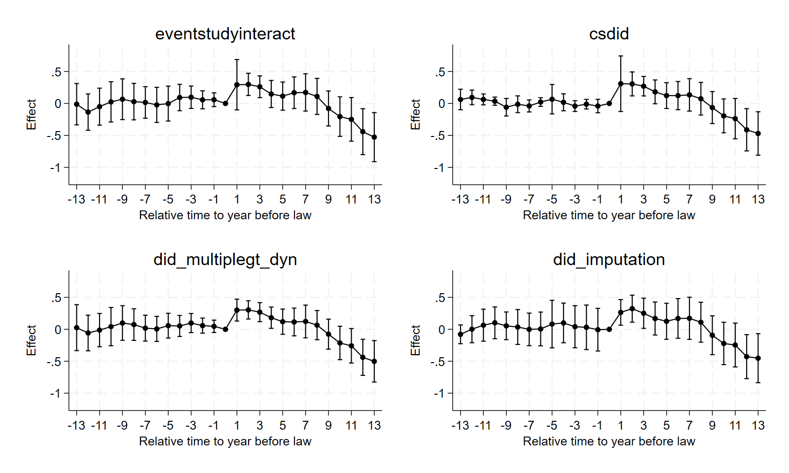
copy "https://raw.githubusercontent.com/Credible-Answers/did_book/main/cc_xd_didtextbook_2025_9_30/Data%20sets/Wolfers%202006/wolfers2006_didtextbook.dta" "wolfers2006_didtextbook.dta", replace
use "wolfers2006_didtextbook.dta", clear

* Panel 1: eventstudyinteract (g1)
use "wolfers2006_didtextbook.dta", clear
replace cohort=. if controlgroup==1
drop if cohort==1956
replace rel_timeminus9=(year==cohort-1-9)
gen rel_timeminus10=(year==cohort-1-10)
gen rel_timeminus11=(year==cohort-1-11)
gen rel_timeminus12=(year==cohort-1-12)
gen rel_timeminus13=(year<=cohort-1-13)
replace rel_time13=(year>=cohort-1+13)
cap drop rel_time14 rel_time15 rel_time16
qui eventstudyinteract div_rate rel_time* [aweight=stpop], absorb(i.state i.year) cohort(cohort) control_cohort(controlgroup) vce(cluster state)

* eventstudyinteract stores its estimates in e(b_iw) and e(V_iw)
matrix b = e(b_iw)
matrix V = e(V_iw)

tempname pf
tempfile coefs
postfile `pf' rel_time coef ci_lo ci_hi using `coefs'
forvalues t = 1/13 {
    local b  = b[1, "rel_time`t'"]
    local se = sqrt(V["rel_time`t'", "rel_time`t'"])
    post `pf' (`t') (`b') (`b' - 1.96 * `se') (`b' + 1.96 * `se')
}
forvalues t = 1/13 {
    local b  = b[1, "rel_timeminus`t'"]
    local se = sqrt(V["rel_timeminus`t'", "rel_timeminus`t'"])
    post `pf' (-`t') (`b') (`b' - 1.96 * `se') (`b' + 1.96 * `se')
}
post `pf' (0) (0) (.) (.)
postclose `pf'

use `coefs', clear
sort rel_time
twoway (rcap ci_hi ci_lo rel_time, lcolor(black)) ///
       (connected coef rel_time, mcolor(black) lcolor(black) msymbol(O)), ///
       title("eventstudyinteract") ///
       xtitle("Relative time to year before law") ///
       ytitle("Effect") ///
       xlabel(-13(2)13) ylabel(-1(.5).5, angle(0)) yscale(range(-1.15 0.8)) ///
       graphregion(color(white)) legend(off) ///
       name(g1, replace)
graph export "figures/ch06_fig63_panel1_eventstudyinteract.png", replace width(1200)

* Panel 2: csdid (g2)
use "wolfers2006_didtextbook.dta", clear
qui csdid div_rate [weight=stpop], ivar(state) time(year) gvar(cohort) notyet agg(event)

tempname pf
tempfile coefs
postfile `pf' rel_time coef ci_lo ci_hi using `coefs'
* Tp0 is the first year of the law, i.e. rel_time = 1
forvalues t = 0/12 {
    local b  = _b[Tp`t']
    local se = _se[Tp`t']
    post `pf' (`t' + 1) (`b') (`b' - 1.96 * `se') (`b' + 1.96 * `se')
}
forvalues t = 1/13 {
    local b  = _b[Tm`t']
    local se = _se[Tm`t']
    post `pf' (-`t') (`b') (`b' - 1.96 * `se') (`b' + 1.96 * `se')
}
post `pf' (0) (0) (.) (.)
postclose `pf'

use `coefs', clear
sort rel_time
twoway (rcap ci_hi ci_lo rel_time, lcolor(black)) ///
       (connected coef rel_time, mcolor(black) lcolor(black) msymbol(O)), ///
       title("csdid") ///
       xtitle("Relative time to year before law") ///
       ytitle("Effect") ///
       xlabel(-13(2)13) ylabel(-1(.5).5, angle(0)) yscale(range(-1.15 0.8)) ///
       graphregion(color(white)) legend(off) ///
       name(g2, replace)
graph export "figures/ch06_fig63_panel2_csdid.png", replace width(1200)

* Panel 3: did_multiplegt_dyn (g3)
use "wolfers2006_didtextbook.dta", clear
qui did_multiplegt_dyn div_rate state year udl, effects(13) placebo(13) weight(stpop) graph_off

tempname pf
tempfile coefs
postfile `pf' rel_time coef ci_lo ci_hi using `coefs'
forvalues t = 1/13 {
    local b  = _b[Effect_`t']
    local se = _se[Effect_`t']
    post `pf' (`t') (`b') (`b' - 1.96 * `se') (`b' + 1.96 * `se')
}
forvalues t = 1/13 {
    local b  = _b[Placebo_`t']
    local se = _se[Placebo_`t']
    post `pf' (-`t') (`b') (`b' - 1.96 * `se') (`b' + 1.96 * `se')
}
post `pf' (0) (0) (.) (.)
postclose `pf'

use `coefs', clear
sort rel_time
twoway (rcap ci_hi ci_lo rel_time, lcolor(black)) ///
       (connected coef rel_time, mcolor(black) lcolor(black) msymbol(O)), ///
       title("did_multiplegt_dyn") ///
       xtitle("Relative time to year before law") ///
       ytitle("Effect") ///
       xlabel(-13(2)13) ylabel(-1(.5).5, angle(0)) yscale(range(-1.15 0.8)) ///
       graphregion(color(white)) legend(off) ///
       name(g3, replace)
graph export "figures/ch06_fig63_panel3_did_multiplegt_dyn.png", replace width(1200)

* Panel 4: did_imputation (g4)
use "wolfers2006_didtextbook.dta", clear
replace cohort=. if cohort==0
qui did_imputation div_rate state year cohort [aweight=stpop], horizons(0/12) autosample minn(0) pre(13)

tempname pf
tempfile coefs
postfile `pf' rel_time coef ci_lo ci_hi using `coefs'
* tau0 is the first year of the law, i.e. rel_time = 1
forvalues t = 0/12 {
    local b  = _b[tau`t']
    local se = _se[tau`t']
    post `pf' (`t' + 1) (`b') (`b' - 1.96 * `se') (`b' + 1.96 * `se')
}
forvalues t = 1/13 {
    local b  = _b[pre`t']
    local se = _se[pre`t']
    post `pf' (-`t') (`b') (`b' - 1.96 * `se') (`b' + 1.96 * `se')
}
post `pf' (0) (0) (.) (.)
postclose `pf'

use `coefs', clear
sort rel_time
twoway (rcap ci_hi ci_lo rel_time, lcolor(black)) ///
       (connected coef rel_time, mcolor(black) lcolor(black) msymbol(O)), ///
       title("did_imputation") ///
       xtitle("Relative time to year before law") ///
       ytitle("Effect") ///
       xlabel(-13(2)13) ylabel(-1(.5).5, angle(0)) yscale(range(-1.15 0.8)) ///
       graphregion(color(white)) legend(off) ///
       name(g4, replace)
graph export "figures/ch06_fig63_panel4_did_imputation.png", replace width(1200)

* Combine the four panels
graph combine g1 g2 g3 g4, cols(2) graphregion(color(white)) name(fig63, replace)
graph export "figures/ch06_fig63_4panel_stata.png", name(fig63) replace width(1600)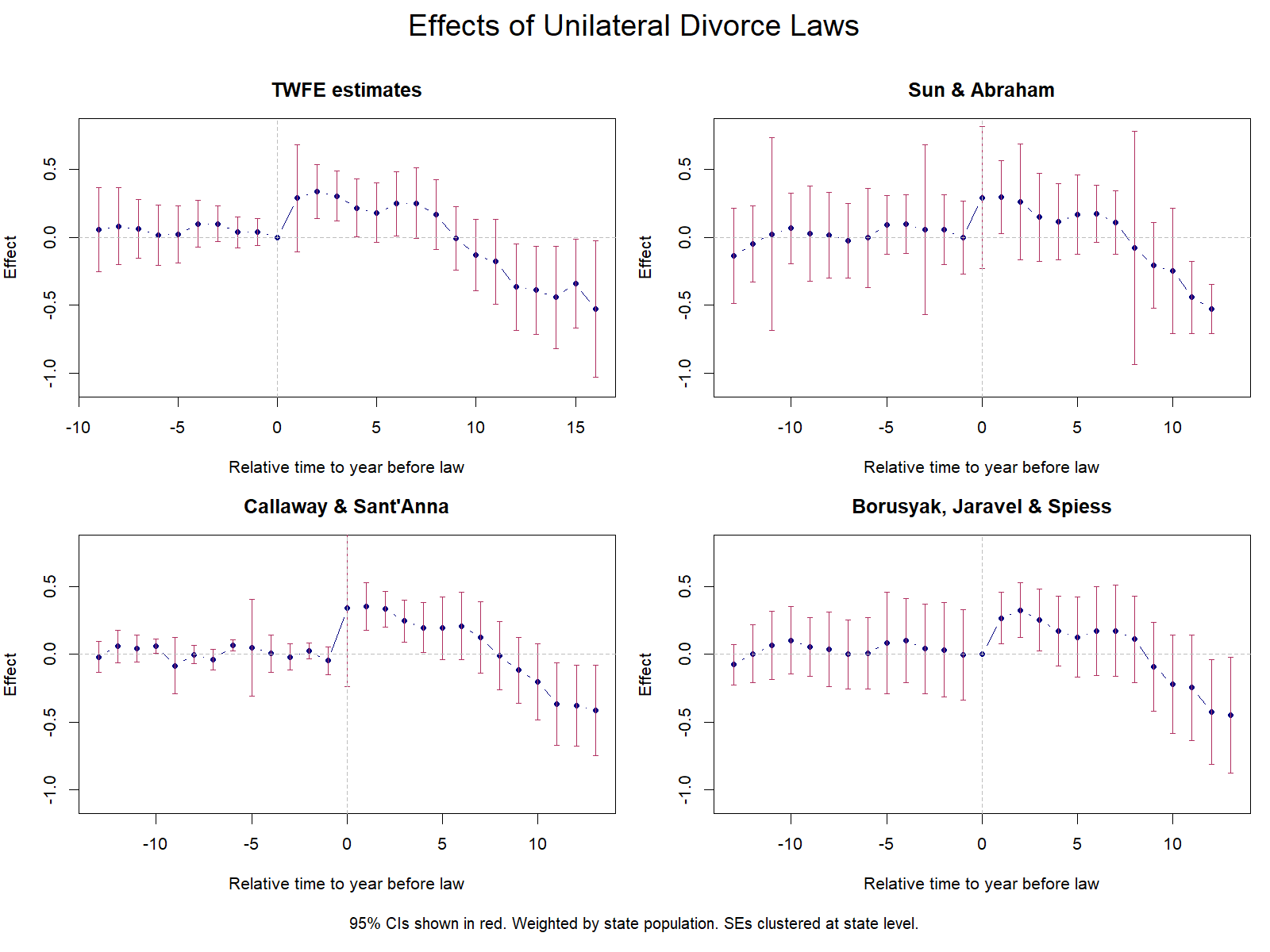
library(haven)
load(url("https://raw.githubusercontent.com/Credible-Answers/did_book/main/cc_xd_didtextbook_2025_9_30/Data%20sets/Wolfers%202006/wolfers2006_didtextbook.RData"))
png(file.path(FIGDIR, "ch06_fig63_4panel_R.png"), width = 1600, height = 1200, res = 150)
par(mfrow = c(2, 2), mar = c(4, 4, 3, 1), oma = c(3, 0, 3, 0))
es_plot(rt_all, co_all, lo_all, hi_all, "TWFE estimates", xlim = c(-9, 16))
es_plot(sa_rt_plot, sa_co_plot, sa_lo_plot, sa_hi_plot, "Sun & Abraham")
es_plot(cs_rt_plot, cs_co_plot, cs_lo_plot, cs_hi_plot, "Callaway & Sant'Anna")
es_plot(bjs_rt_plot, bjs_co_plot, bjs_lo_plot, bjs_hi_plot, "Borusyak, Jaravel & Spiess")
mtext("Effects of Unilateral Divorce Laws", outer = TRUE, side = 3, cex = 1.5, line = 1)
mtext("95% CIs shown in red. Weighted by state population. SEs clustered at state level.",
      outer = TRUE, side = 1, cex = 0.8, line = 1)
dev.off()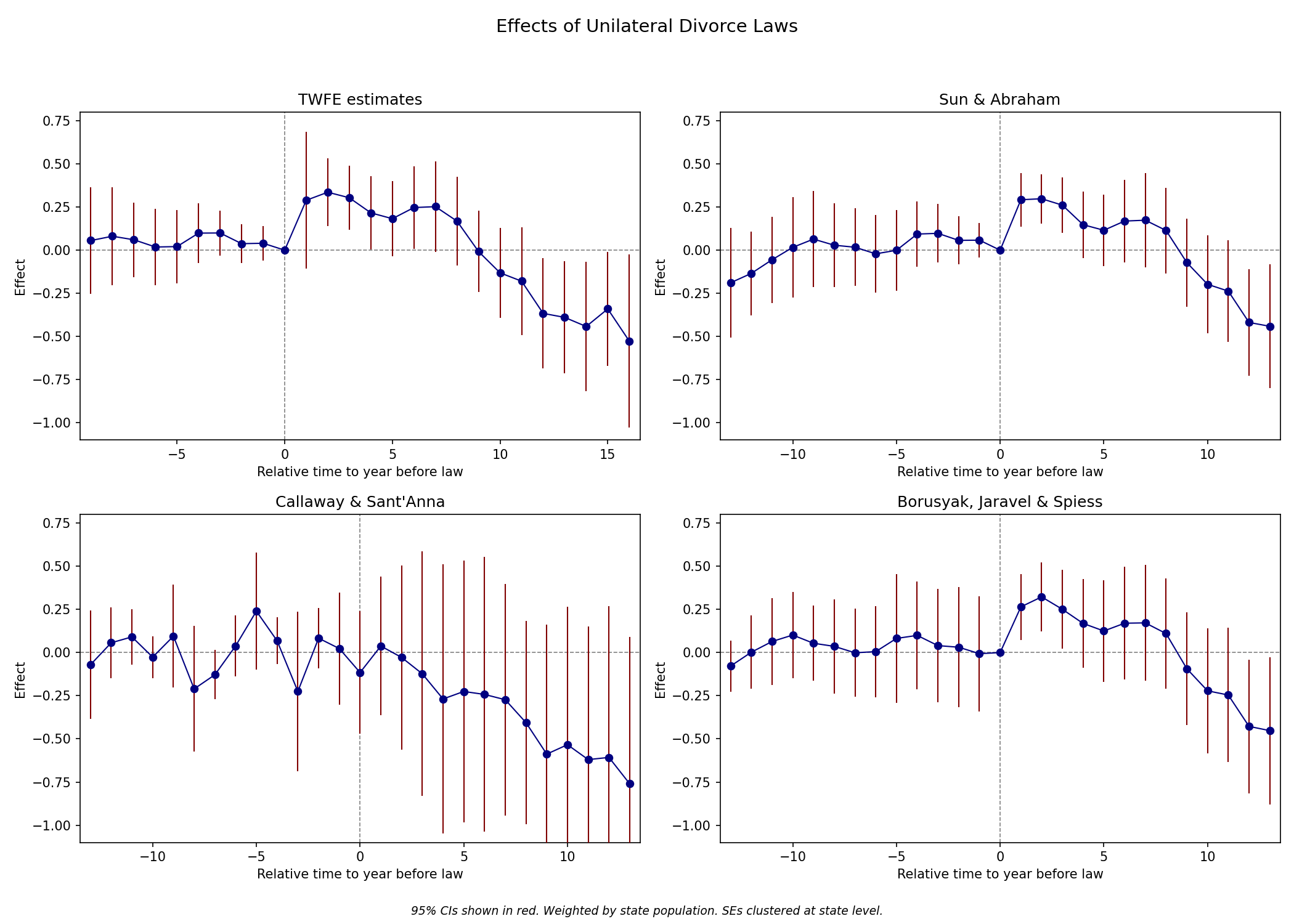
import pandas as pd
df = pd.read_parquet("https://raw.githubusercontent.com/Credible-Answers/did_book/main/cc_xd_didtextbook_2025_9_30/Data%20sets/Wolfers%202006/wolfers2006_didtextbook.parquet")
fig, axes = plt.subplots(2, 2, figsize=(14, 10))
es_plot(axes[0, 0], rt_fig62, co_fig62, lo_fig62, hi_fig62, "TWFE estimates", xlim=(-9.5, 16.5))
es_plot(axes[0, 1], sa_rt, sa_co, sa_lo, sa_hi, "Sun & Abraham")
es_plot(axes[1, 0], cs_rt, cs_co, cs_lo, cs_hi, "Callaway & Sant'Anna")
plt.suptitle("Effects of Unilateral Divorce Laws", fontsize=14)
fig.text(0.5, 0.01,
    "95% CIs shown in red. Weighted by state population. SEs clustered at state level.",
    ha='center', fontsize=9, style='italic')
plt.tight_layout(rect=[0, 0.03, 1, 0.95])
plt.savefig(FIGDIR / "ch06_fig63_4panel_Python.png", dpi=150)